Modelling a mechatronic system and being able to simulate the dynamic behaviour with analysis methods in frequency and time domain gives us deep insight into the properties and performance of the system. However, nice animations and graphics do not necessarily mean that the results are practically usable. What if the model does not match reality well enough?
Can I actually trust a dynamic model?
Well, there is no universal answer to this question. To judge the accuracy of a model is usually the aim of model validation using measurements. However, this blog post is not about validation, but instead shows an example of the extent to which a dynamic model can typically represent reality when nothing has gone wrong. It is good to get an idea of how close you can get with the models.
The results shown below are the results of a model without specific parameter tuning. Stiffness values for linear guides are taken from the supplier, default damping values are used, and the geometry has even been partially measured and redrawn due to missing CAD files. Only static friction of linear guides was measured; by means of a spring scale.
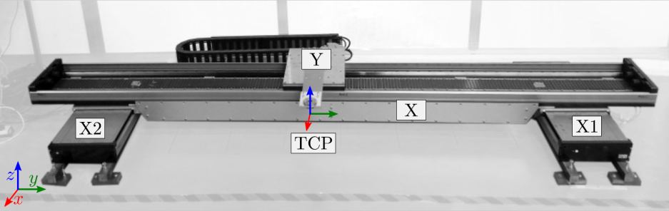
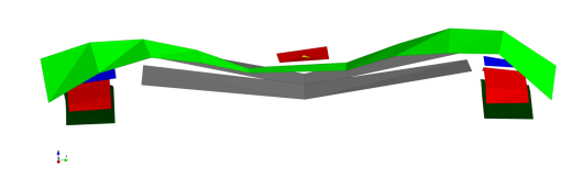
We discuss an example comparison between simulation and measurements conducted on our dynamics test bench shown in Figure 1. This is a 2D gantry stage driven by linear direct drives.
Figure 1: Dynamic test bench Andromeda - Gantry positioning system located at Technopark Zurich
We discuss results of three different kinds:
Modal analysis of the uncontrolled structure
Open- and closed-loop frequency response functions (FRFs)
Contour error for dynamic set points
Modal analysis
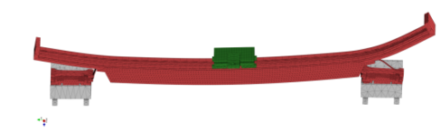
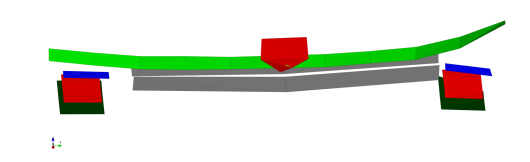
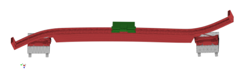
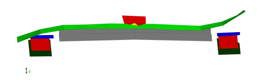
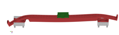
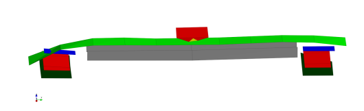
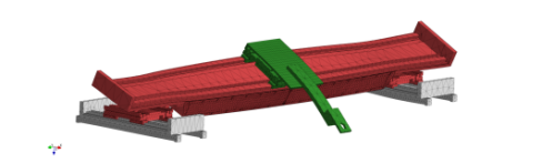
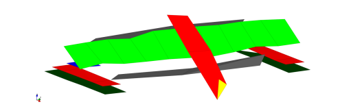
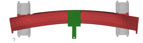
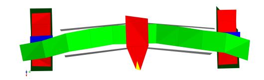
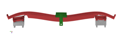
We performed an experimental modal analysis (EMA) on the uncontrolled structure, i.e. with disabled controllers. This gives a deep insight in the vibration properties of the system and allows for a good comparison between the modelled and the real structure. The results for the first six modes are shown in Table 1.
Simulation
Experimental modal analysis (EMA)
Deviation
Frequency [rad/s]
Mode shape
Frequency [rad/s]
Mode shape
Rel. deviation [%]
226
231
2.2
291
307
5.2
308
329
6.4
373
368
-1.4
753
828
9.1
784
828
5.3
Table 1: Comparison of mode shapes and frequencies in simulation and measurement
The simulated mode shapes correspond very well to the ones from the EMA and the eigenfrequencies show an error below 10 %. This kind of measurements is very useful for the identification of weaknesses and errors in the structural model.
There is a short anecdote about the modal analysis of this system. Actually, after having performed the first EMA and comparing with simulation, the results did not match at all. Especially a transversal displacement mode in Y direction was off in frequency and shape. We distrusted the model and after days of unsuccessful model modification and parameter tuning, we got back to the machine. After taking a closer look, we recognised that some screws of the machine support had come loose. We tightened the screws, redid the EMA and got the results above. This shows, that one has to consider both the experimental and simulation setup if the results of both do not match.
Open- and closed-loop frequency response functions
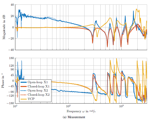
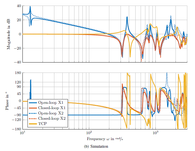
Let’s go a step further and include the axis controllers in the model. Figure 2 shows velocity Bode diagrams for the X axis (X1 and X2 drives) for both, open and closed loop. Additionally, the behaviour at the tool centre point (TCP) is shown for the closed-loop case. Besides internal encoders (glass scales) also a Heidenhain KGM grid encoder was used in order to measure the response at the TCP.
Figure 2: Comparison of open- and closed-loop velocity Bode diagramms of the X-Axis in simulation and measurement
The figure shows that the most important behaviour including the overshoot at the TCP as well as the damping introduced by the drives (from the blue to the red curve) match well.
Contour error for dynamic set points
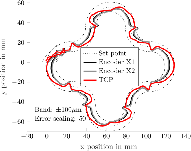
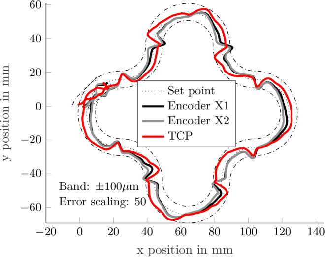
In order to get a more intuitive result on how the model matches reality, we also conducted a path tracking experiment with a dynamic contour. Figure 3 shows the results as contour error plots with errors scaled by a factor of 50 (normal to the path direction). The measurements at the TCP were taken using a KGM grid encoder.
Simulation
Measurement
Figure 3: Comparison of contour errors in simulatino and measurement
The results show how well a dynamic model created in MORe can represent reality. These plots show
dynamic controller errors at the curvature reversal points (transition from one circle segment to another),
oscillation of the TCP after curvature reversal points,
quasi-static deviation between TCP and axis encoders, and
backlash effects due to static friction.
All these effects, even though not perfect, match very well between measurement and simulation both qualitatively and quantitatively. The maximum measured contour error at the TCP is 105 µm and corresponds well with the maximum contour error from simulation, which is 113 µm. The maximum encoder contour errors are 114 µm and 129 µm for measurement and simulation, respectively.
Animation 1: Control deviation and structural deformation during travel on a section of the contour of Table 2
Now the nice thing about simulation. You can get a deeper insight in what is actually going on. Let’s have a closer look at what happens in the structure when the axes follow the contour from Figure 3. Animation 1 shows the errors exaggerated by a factor of 1000. We see the quasi-static deformation caused by acceleration of the axes, we also see the vibration after dynamic excitation at the curvature reversal points.
Conclusion
This example shows that a model can replicate the most important dynamic behaviour of a mechatronic system pretty well, also without tuning parameters to measurements. This does not mean that no measurements are required at any stage in the modelling and development process. Validation measurements are mandatory in order to learn more about the models and their accuracy. Every model that has been validated generates knowledge about strengths and weaknesses of the models that can directly be used for the next model. Thus, with every machine generation, the model can be used to predict the final behaviour more accurately. This holds especially if similar components and manufacturing processes are used for the different machines.
We started this blog with the question if you can trust a dynamic model. Yes, you can. However, you should validate it first.
Take-home message
MORe models can replicate the dynamic behaviour of a mechatronic system quite well, also without parameter tuning. However, in order to improve both the accuracy of simulations and the level of trust in the models, every model should be validated with measurements as soon as they are available.
References
D. Spescha, S. Weikert, K. Wegener. (2020) Simulation in the Design of Machine Tools. In: Yan XT., Bradley D., Russell D., Moore P. (eds) Reinventing Mechatronics. Springer, Cham, http://dx.doi.org/10.1007/978-3-030-29131-0_11