Tutorial

This tutorial is based on MORe version 1.2.5.

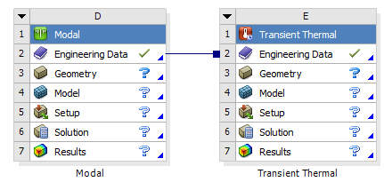
ANSYS

1. The modeling process begins with simplifying the geometry in CAD. This is necessary in order to reduce the amount of mesh elements needed in the FE model. Alternatively, simplification can also be accomplished with the SpaceClaim modeler from ANSYS.

2. Launch ANSYS Workbench and create a new modal analysis.

3. Import the simplified CAD geometry by right clicking on the Geometry tab of the modal analysis.

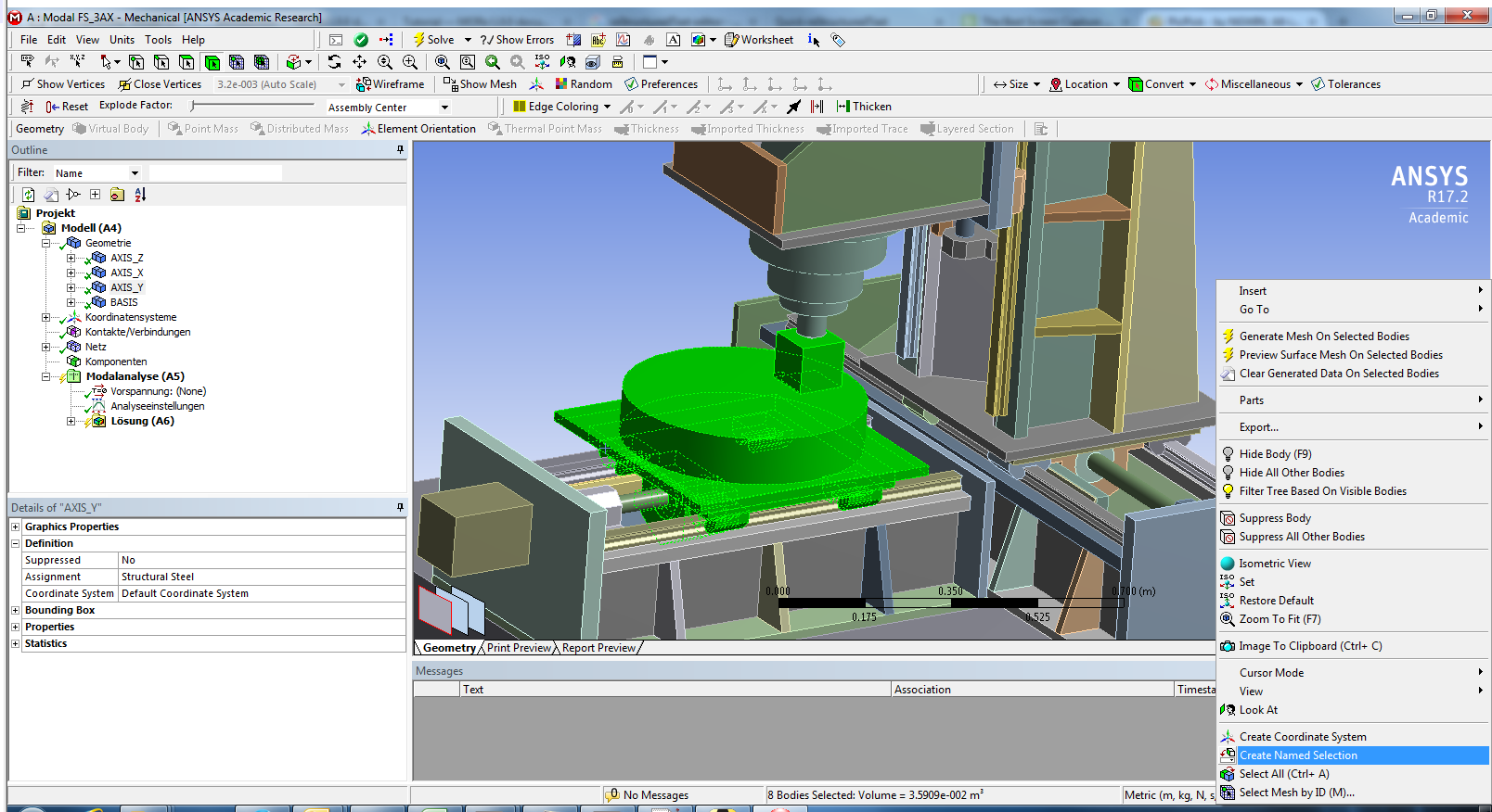
4. Now open ANSYS Mechanical by double clicking on the Model Tab of the modal analysis. Now we need to divide the machine model into components. A component consists of all bodies, that move together as e.g. an axis or the machine basis. This results in a component for each axis and one for the base. If ball screws are used for the axis movement, a separate component for each ball screw spindle has to be created. Select all moving bodies of the Y-axis. Open the context menu by right click and select Create Named Selection and name it Y-axis. Repeat this step for all axes (and ball screw spindles).

   
   
   

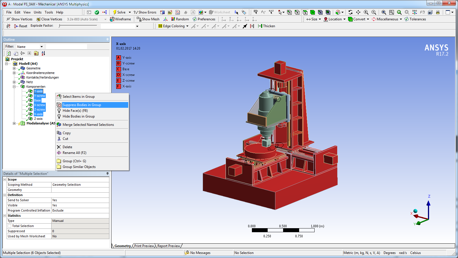
5. For a better overview, the components we are not working on can be suppressed. Select the components and open the context menu by right-clicking, select Suppress Bodies in Group.

   
   
   

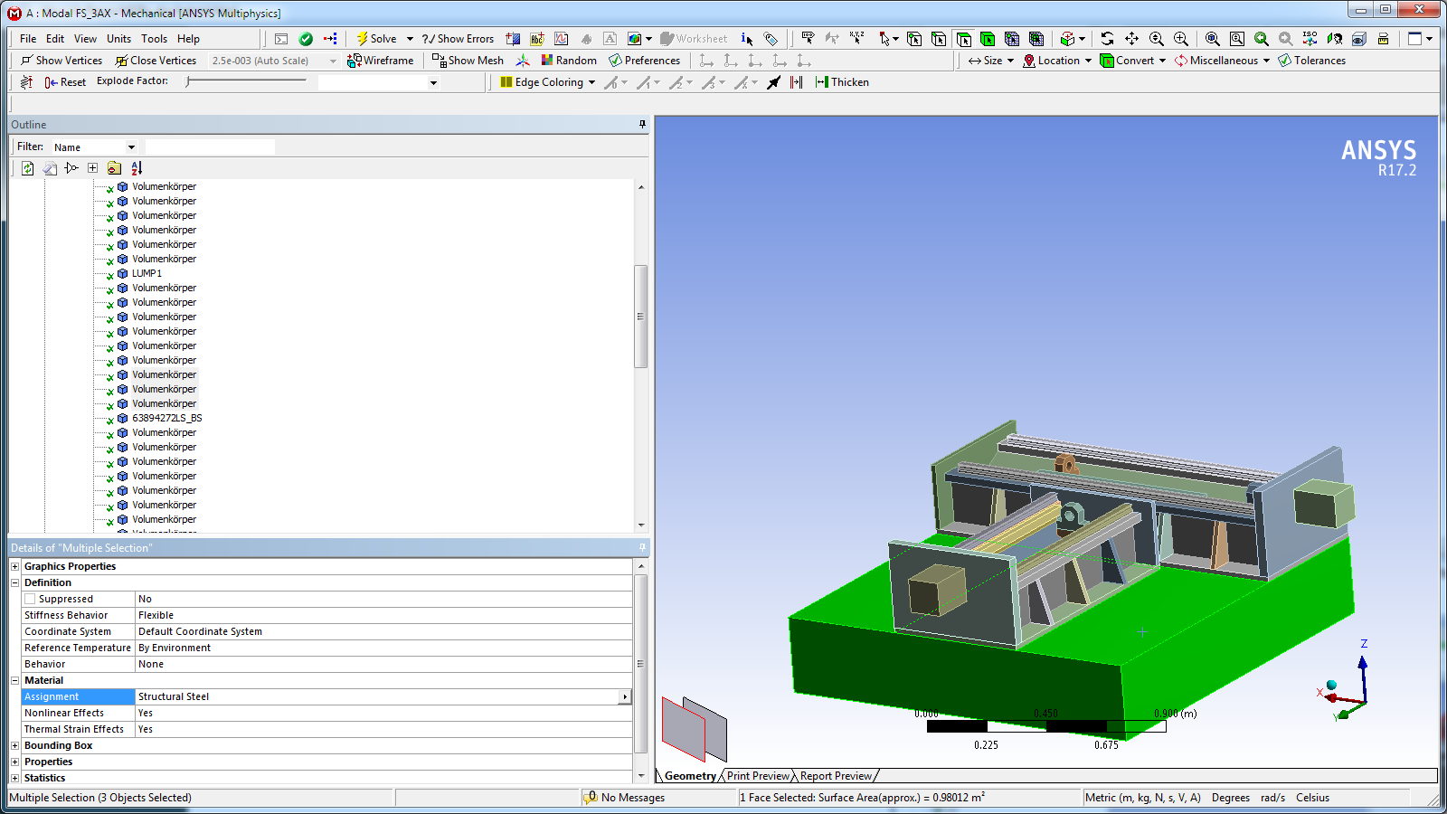
6. Each body in the model needs material properties. To assign the properties, select a body (or multiple) and select the desired material in the Assignment box on the bottom left.

   
   
   

7. The modal analysis only supports the coefficient of thermal expansion as thermal property. To add additional thermal information to the material properties, add a thermal transient analysis to the project and link the engineering data of both analyses. The thermal properties of the selected material can now be changed by clicking on engineering data.

   
   
   

8. In the next step we define contacts between all bodies (parts) of a component. Highlight Contacts in the model tree then select Contact in the top panel to create a new contact. Now select the two faces that are in contact, one for Contact and one for Target. Repeat until all contacts of each component are defined. However, do not create contact between components, as each component has to be free in space.

   
   
   

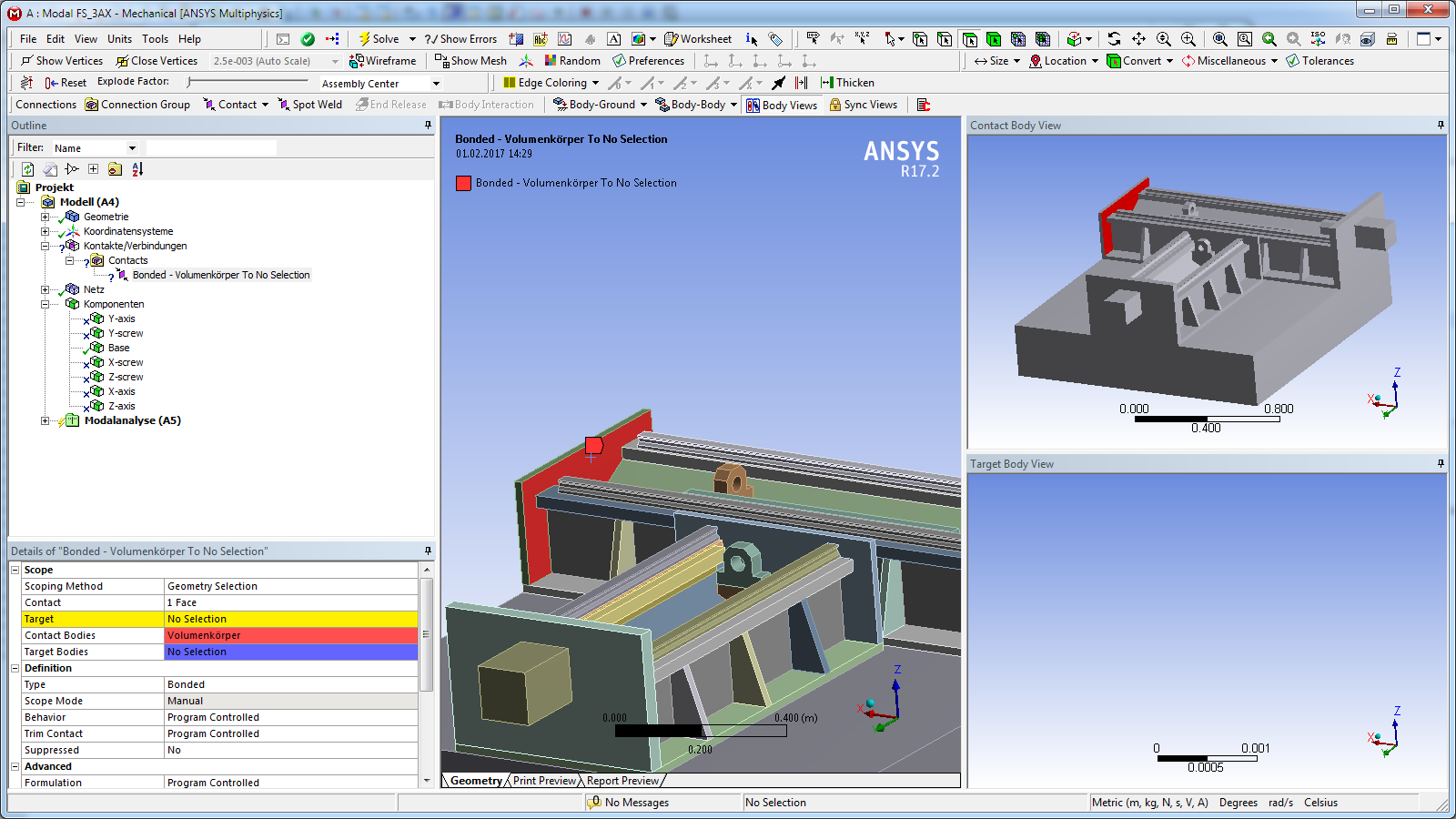
9. Next, we need to generate the mesh for the FE analysis. Right-click on Mesh in the tree and select Generate Mesh. Depending on the geometry of the parts, it might be necessary to define finer mesh on some parts. This can be accomplished by using Mesh Control in the top tool bar. However keep in mind, that using finer mesh increases the amount of mesh elements. The speed of the following process of model order reduction depends heavily on the amount of mesh elements, which makes meshing a balance between speed and accuracy.

   
   
   

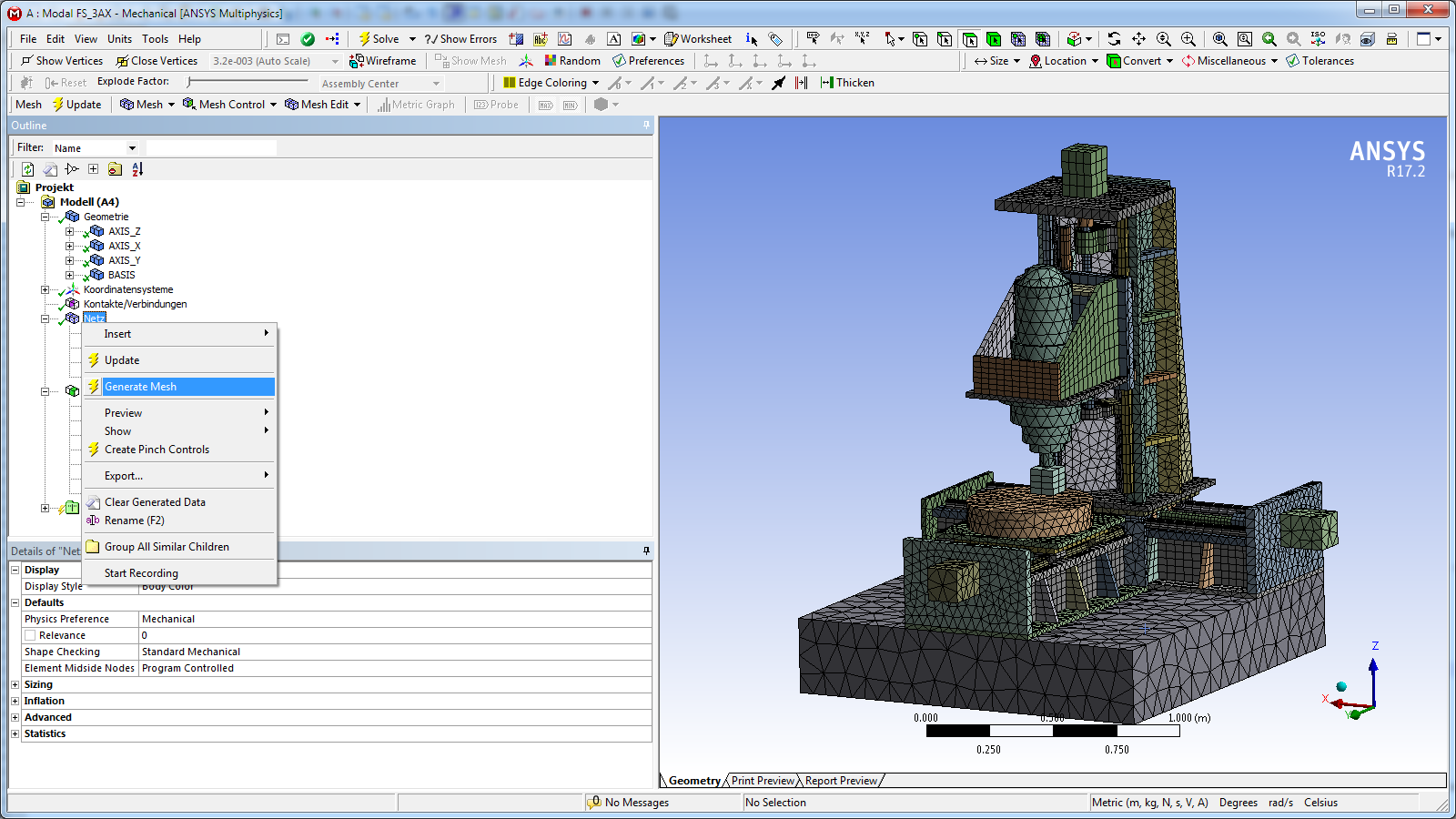
10. To check that no contacts are missing, it is good practice to solve a modal analysis for each component. Suppress all but one component (explained in step 5). Now right-click on Modal Analysis in the tree and select Solve from the context menu. When the solving process is completed, click on Solution in the tree. In the table on the right hand side select all modes. Use Create Mode Shape Results in the context menu. Right-click on Solution in the tree and select Evaluate all Results. If all contacts were defined correctly the component has 6 rigid body modes (the frequency of the first six modes is close to 0Hz). Also check the mode shapes for missing/incorrect contacts. Repeat for each component.

    
    
    

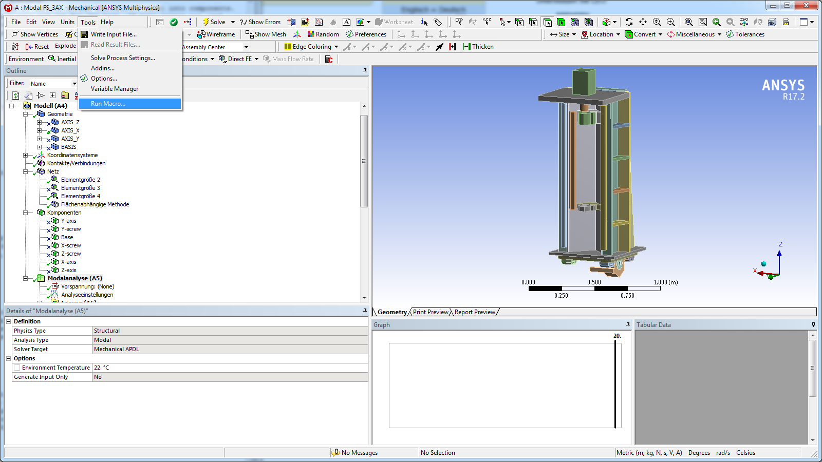
11. Now the model is ready to be exported for MORe. As each component has to be exported separately, suppress all but one component. Click on Modal Analysis in the tree to highlight it. Now click on Tools in the top menu bar and select Run Macro…. Navigate to the folder where MORe is installed (e.g. C:/Simulation/MORe) then navigate to the sub-folder /src/ansys and select exportForMORe. Click yes on the dialog box. When the export process is completed, a windows explorer window will pop up. Select all the files with the name with MORe.* and copy them to a folder named after the component exported (e.g. C:/Simulation/Machine1/Ansys_exports/X_Axis). Repeat for each component (the exported files for the Y-axis component are copied to /Ansys_exports/Y_Axis, and so forth)

    
    
    

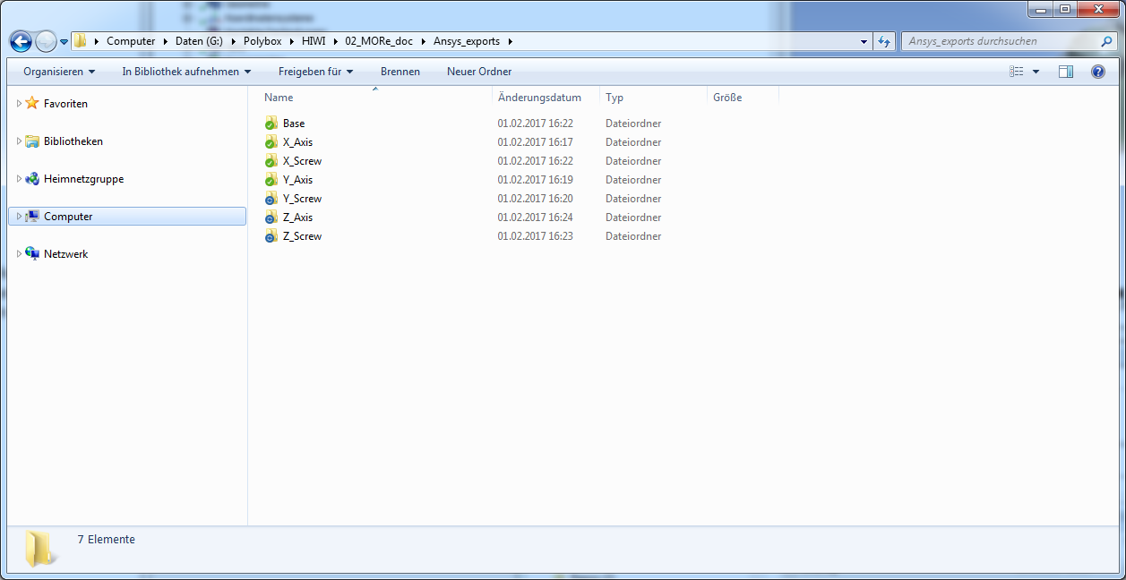
12. You should now have a folder containing one sub-folder for each component of the model. Each sub-folder contains the exported component from Ansys (MORe.mass, MORe.stiff, MORe.mapping, MORe.topo, MORe.cdb).

    

MORe

Startup

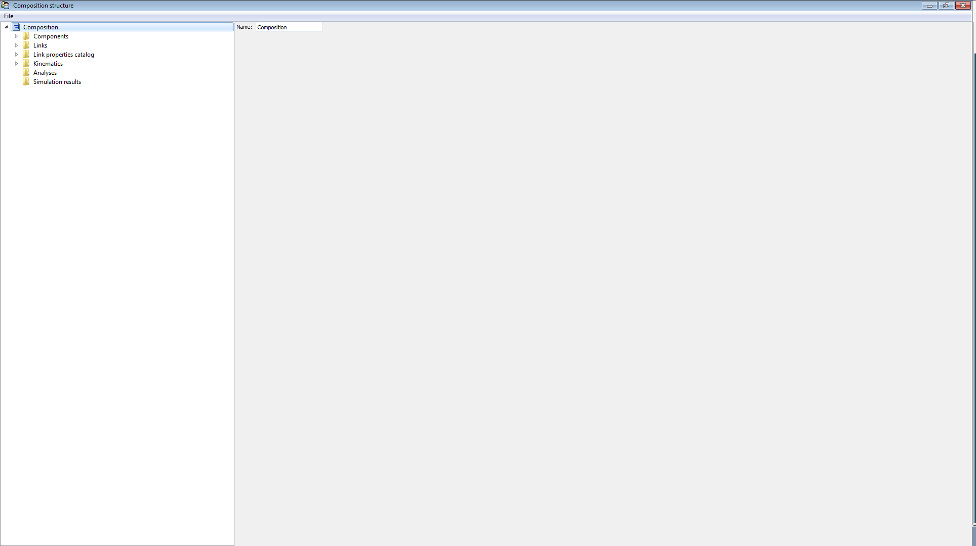
1. Now we are ready to start in MORe. Navigate to the folder /MORe/src/python/startup (e.g. C:/Simulation/MORe/src/python/startup). Double click the MORe.bat file to start MORe. If everything was installed correctly (refer to the Chapter Installation) the MORe GUI appears after a few seconds.

   

Import Components

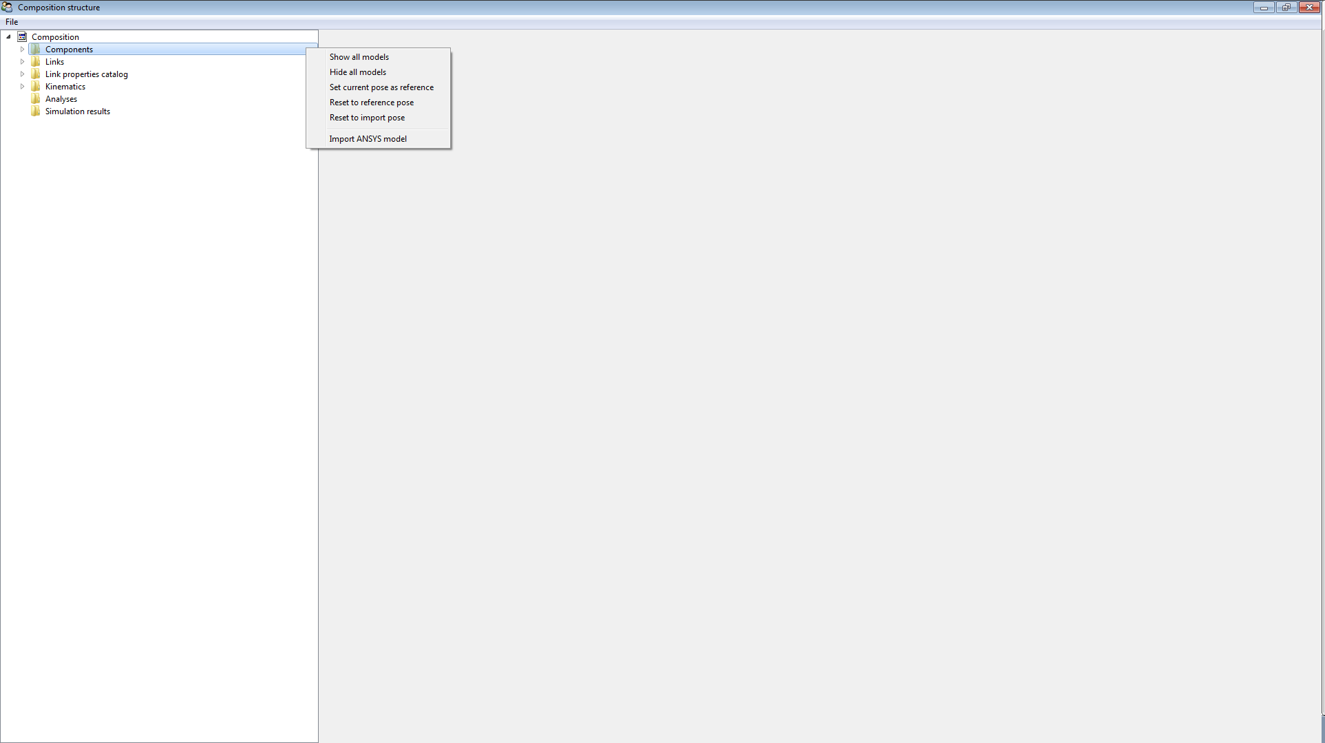
1. Next we import the Components from the Ansys model. In the tree of the MORe-GUI right-click on Components and select Import ANSYS model. In the dialog box navigate to the folder where your Ansys exports are (e.g. C:/Simulation/Machine1/Ansys_exports) and enter the sub-folder for a component (e.g. the Base) and select the MORe.cdb file. click Open. Depending on the model size (number of mesh nodes) the import process may take a few minutes.

   
   
   

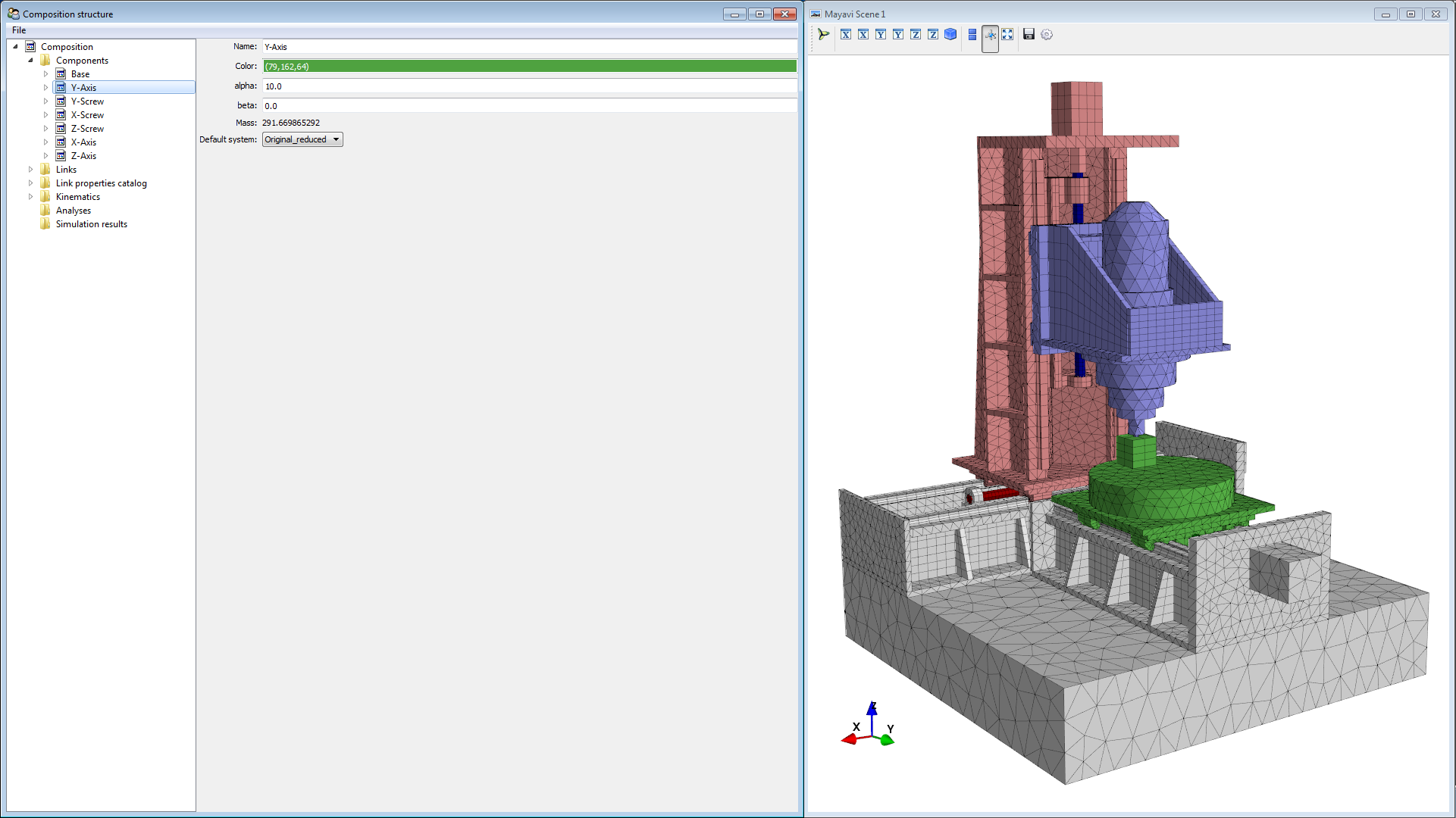
2. When the import is finished, a graphics window displaying the imported component shows up. Rename the component to a more meaningful name (e.g. Base). Repeat the process for each component of the model.

   
   
   

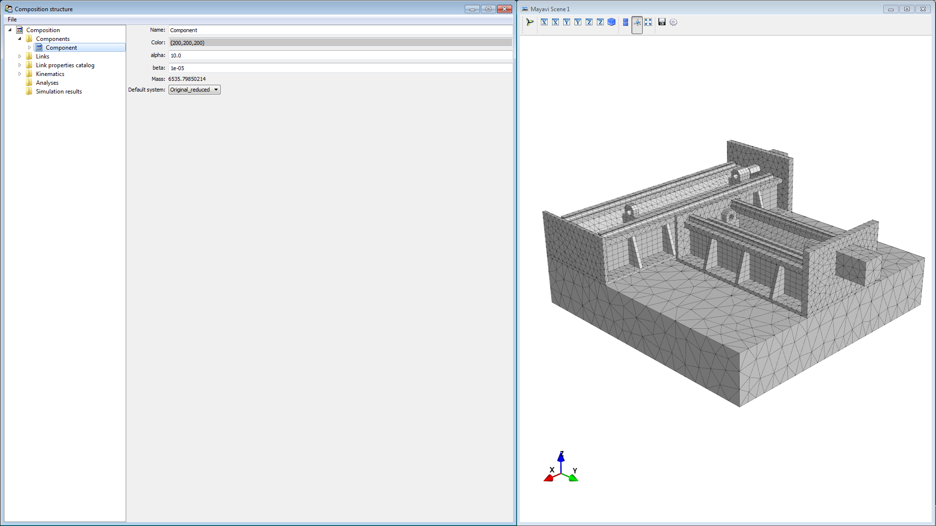
3. For a better overview you can change the color of the components. Now it’s time to save your progress. Use File -> Save as . Note: saving takes some time (depending on model size), however you should save from time to time. If you have enough space on your hard drive, it is recommended to create a new file each time you save and not to overwrite the old one just to ensure that there is an older file in the case that a crash during the save process would leave a corrupted file.

   
   
   

Interfaces

MORe has basically two different types of interfaces:

• stationary interfaces

• moving interfaces

Each interface has 6 degrees of freedom, 3 translations and 3 rotations. We need interfaces for linking the components together. Therefore we have to define an interface on each side of the contact zone. This means we usually define interfaces for:

• linear guides (carriage and rail)

• bearings (inner and outer ring)

• ball screws (nut and spindle)

Interfaces are also used to evaluate displacements and apply external loads, therefore we also define interfaces for

• measuring scale (scale and encoder head)

• tool center point (TCP)

• workpiece

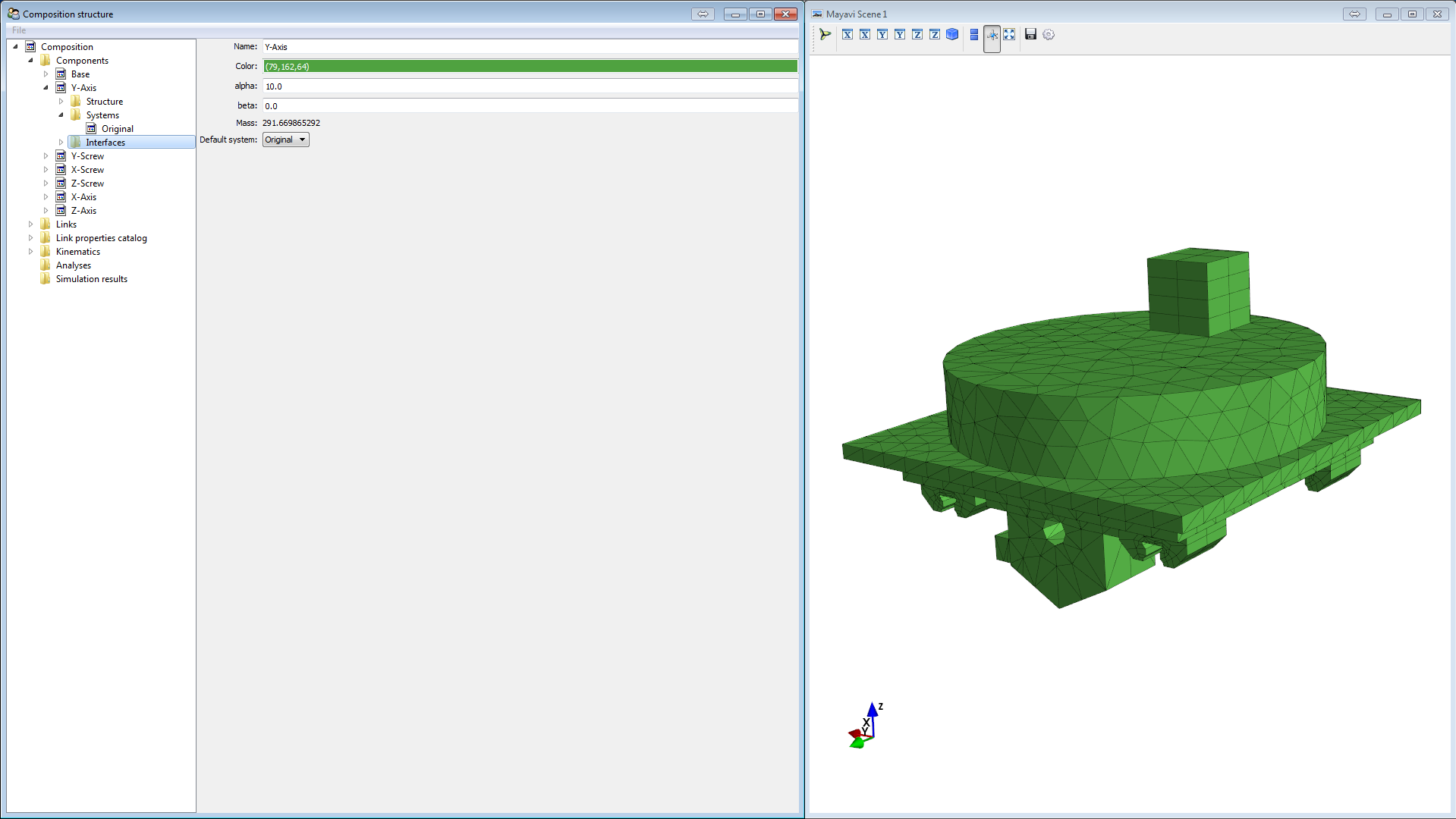
1. We start defining interfaces for the Y-Axis component. To make the process easier, we hide all the other components by right-clicking on them in the tree and selecting Hide Model. Now expand the tree for the Y-Axis by clicking on the triangle next to it. To create a new interface right-click on the Interfaces entry and select New 6dof interface.

   
   
   

2. This will create a new entry called * interface. This will be an interface for one of the carriages, thus we rename it to Y_carriage_11 (_11 because it is the first carriage in x and the first in y direction).

   
   
   

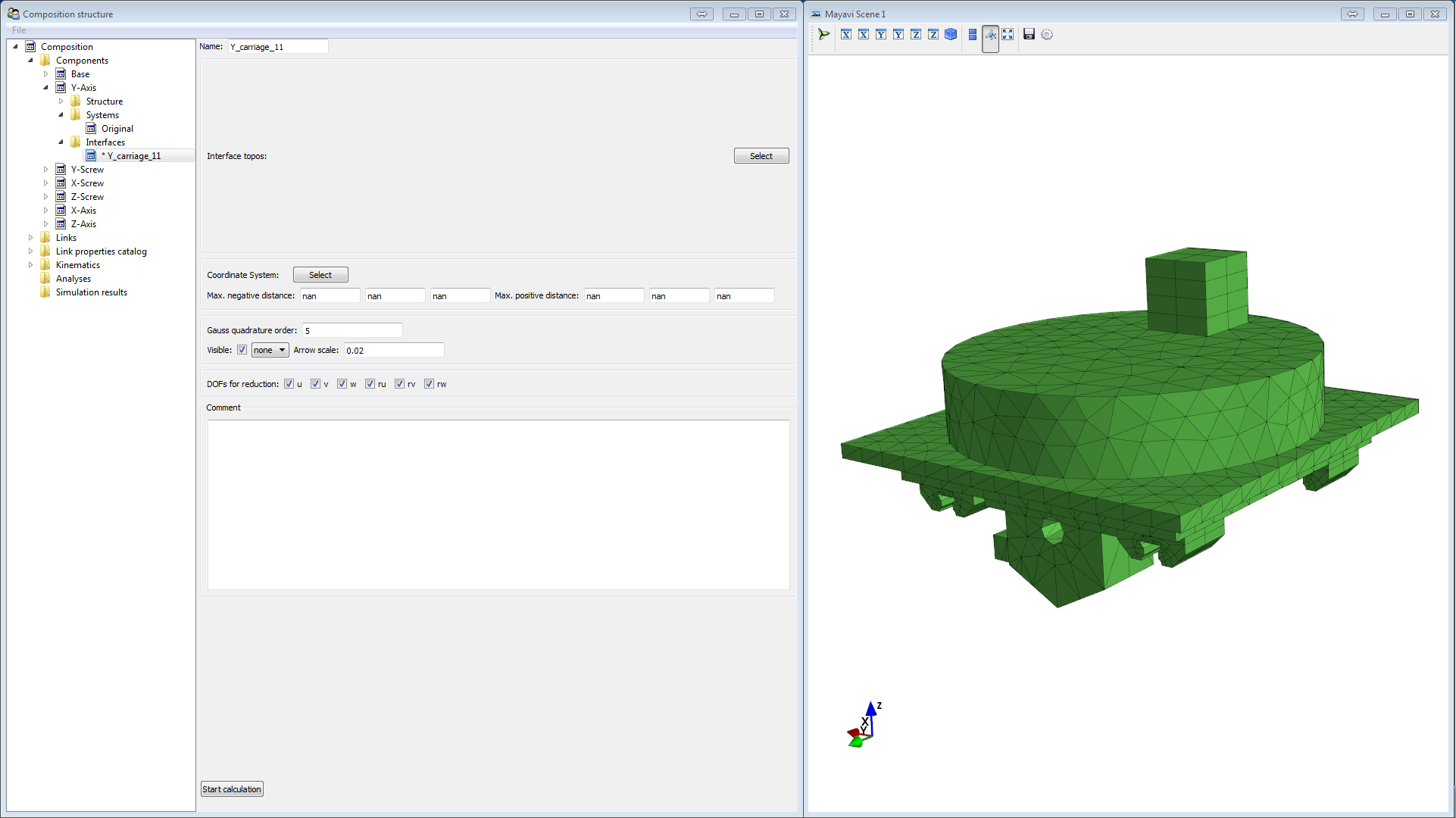
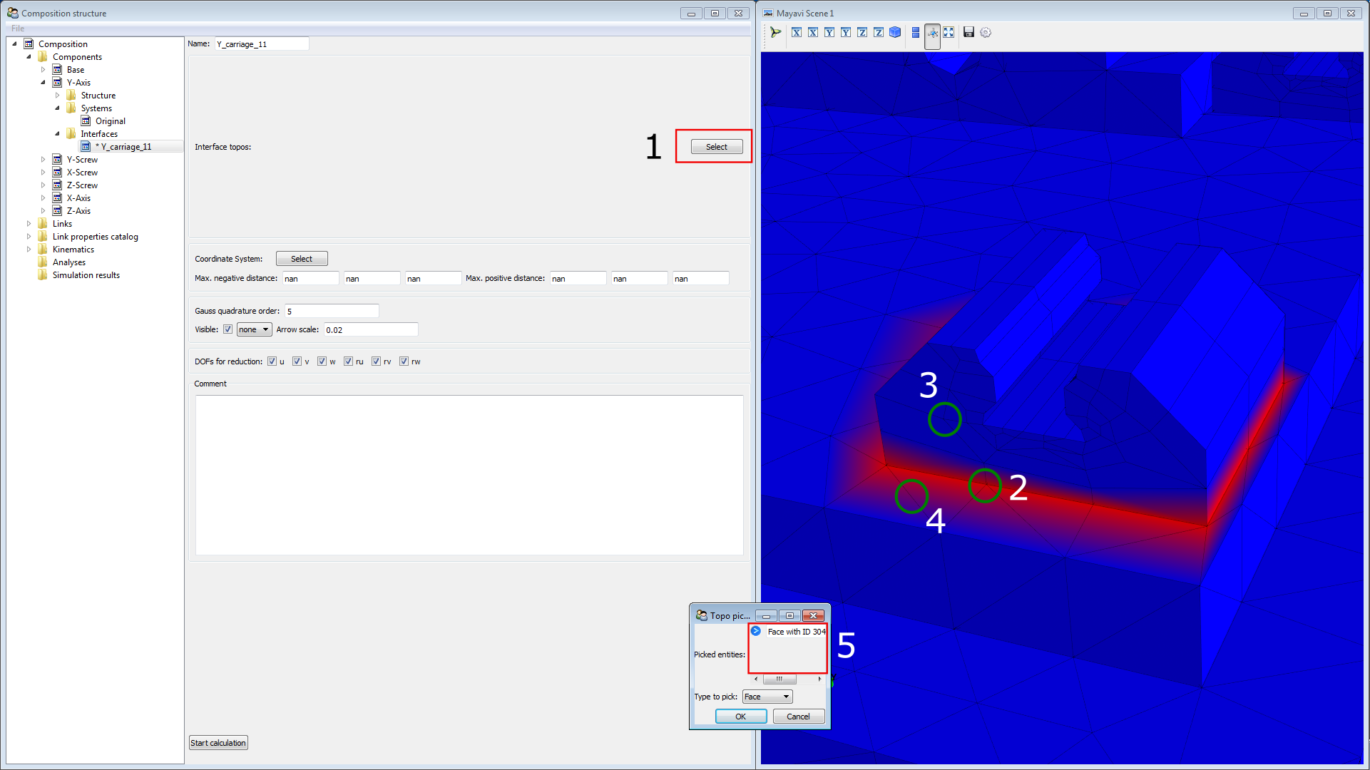
3. Now we have to define to which faces the interface will be attached. Click on the Select Button in the Interface topos box (1). A small box (called Topo-picker) opens in which we can select what type of topology we want to select. Since we want so select faces we leave it on default. We want to select the face on which the carriage is connected to the slider. Since this face is hidden we need a little trick to select it. Click on the node that is part of the face (2), this will select all faces the node is part of. Now click on the faces (3) and (4) to deselect them. In the Topo picker box check that only one face is picked (5). Then click OK.

   
   
   

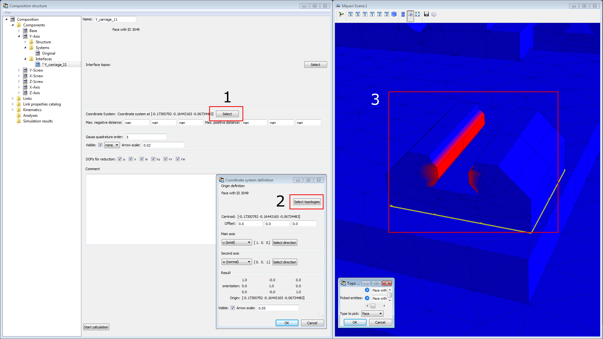
4. Next we need to define a local coordinate system for the interface. Click on the Select button next to Coordinate System (1). This will open the Coordinate system definition dialog-box and it will display a coordinate system in the graphics window (with following colors: axial:red, transversal:green, normal:blue). We want the coordinate origin to be between the faces that are in contact with the rail. Therefore we need to select which faces define the origin. Click Select topologies (2). Now the Topo-picker opens. Deselect the face that is currently selected and the select the two faces displayed in the picture (3). Click OK.

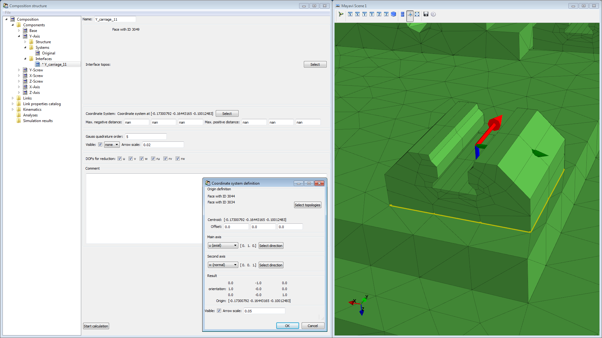
5. Finally we need to define the orientation of the coordinate system. We define axial in direction of motion (+Y for this carriage), and normal in normal direction of the rail (+Z for this carriage). To change the orientation click Select direction. For axial type 0.0 : 1.0 : 0.0 in the dialog box. The normal direction is already correct.

   
   
   

6. Click on Start calculation in order to invoke the calculation of nodal weights for the specific force distributions. An interface that is up-to-date has no asterisk prefix in the name, an interface with a asterisk has to be updated.

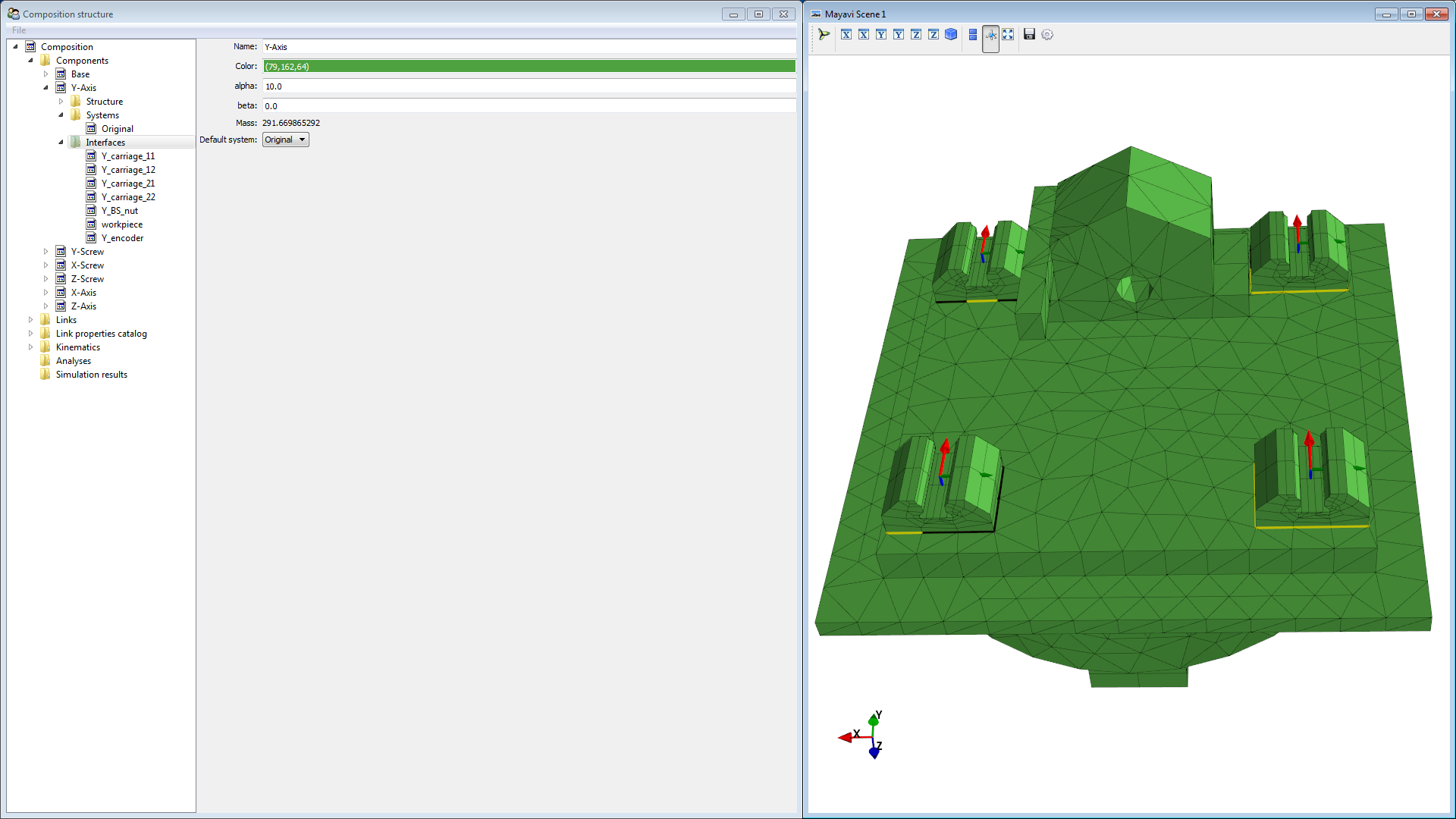
7. Repeat for the remaining carriages on the Y-Axis. When done the graphics windows should display all the interfaces in correct orientation. If a interface is not displayed, click on in in the tree to show it.

   
   
   

8. Create a new 6dof interface for the ball screw nut with the bore mantle surface as topology for the interface as well as for the coordinate system. Define the coordinate system in the same orientation as the carriages.

   
   
   

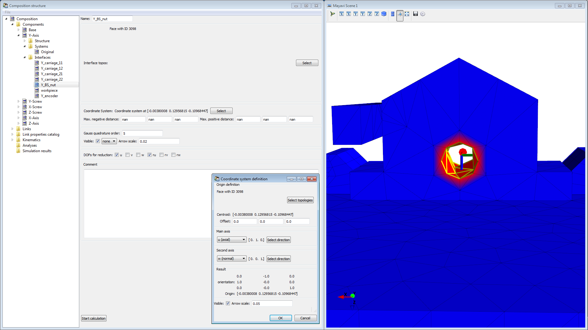
9. Since the nut will transmit forces in u (axial) direction and torque in ru direction only, we deselect the other direction from DOFs for reduction. Rename it to Y_BS_nut.

10. Create a new 6dof interface for the encoder head. Configure the u-direction of the coordinate system in y-directon.

    
    
    

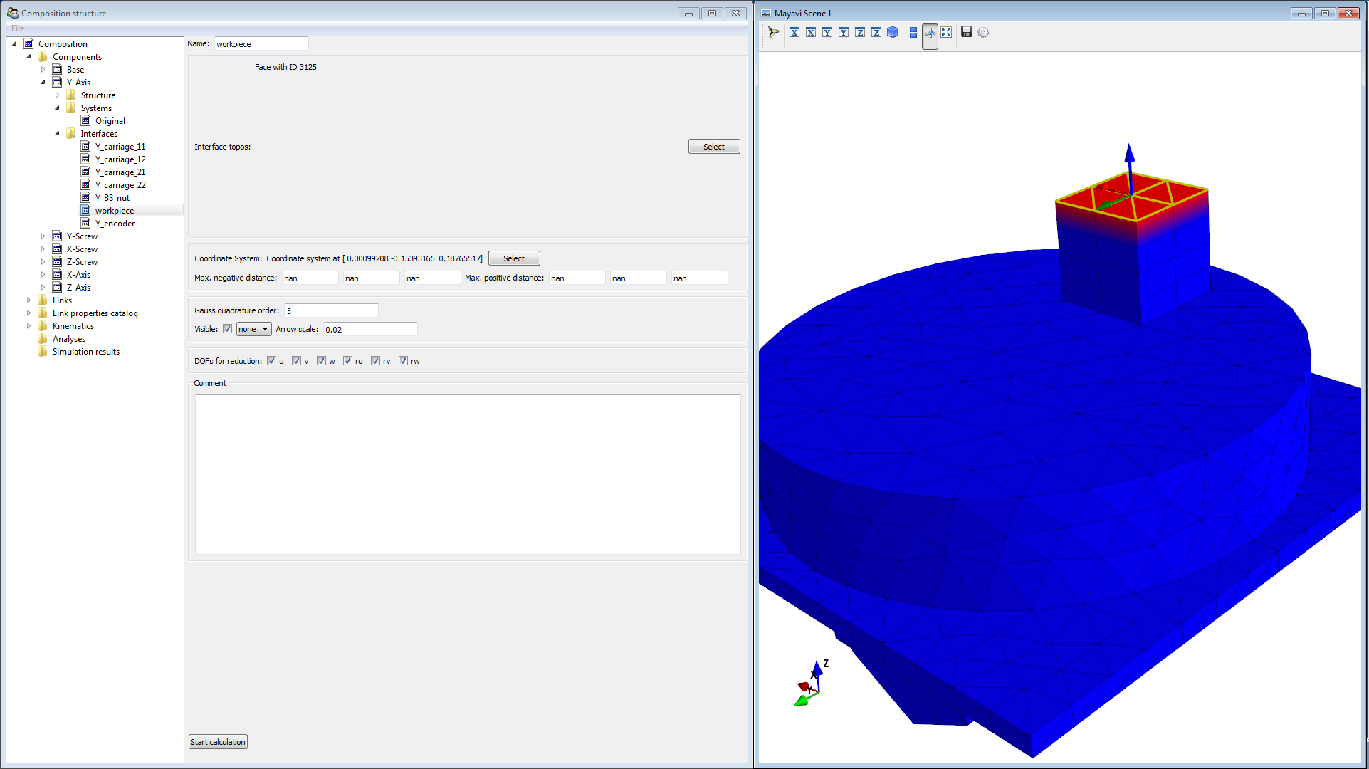
11. Create a new 6dof interface for the workpiece. For the coordinate system orientation use the global system.

    
    
    

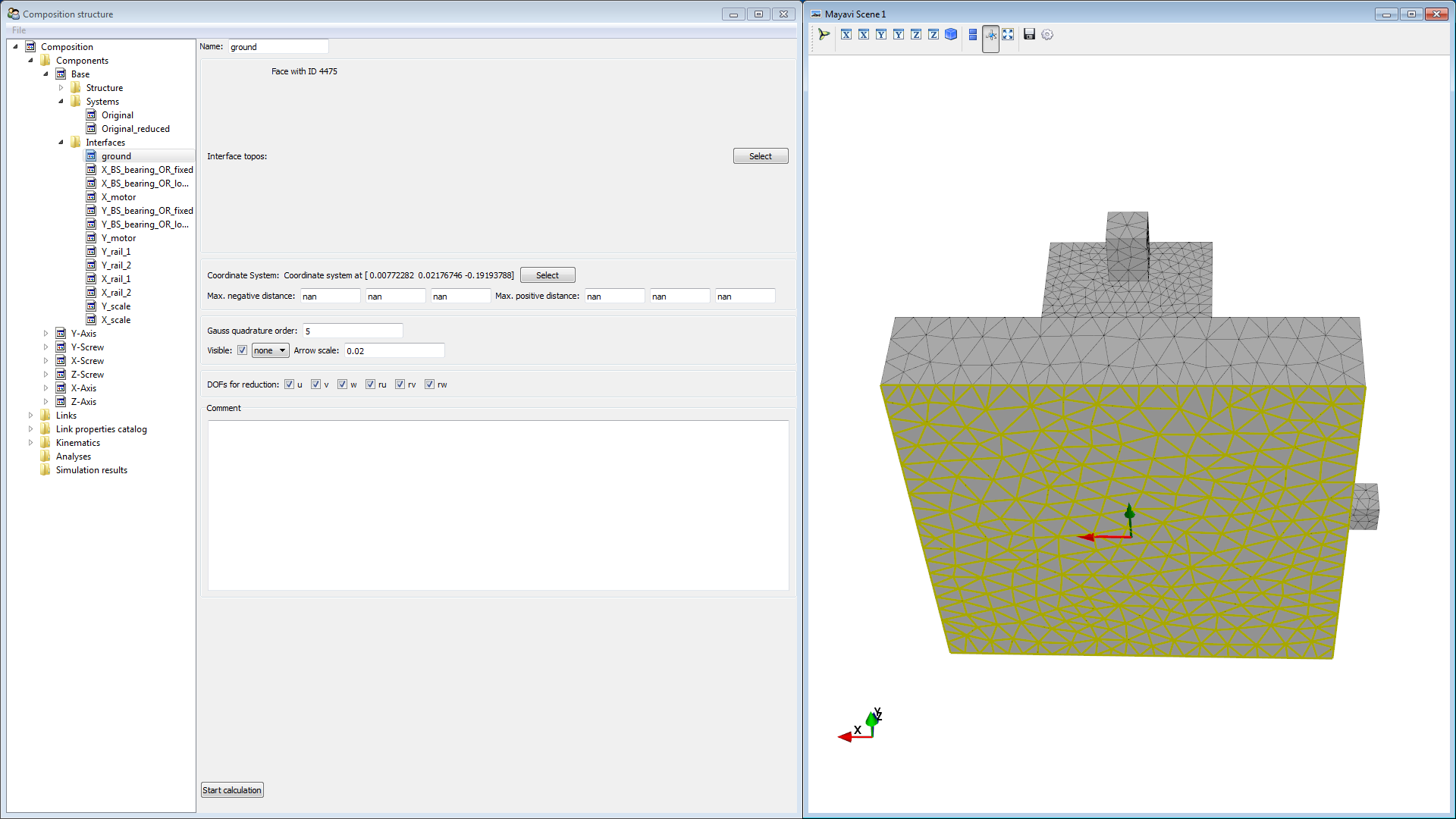
12. Next we will work on the Base component. Hide the Y-Axis and show Base (use the right-click context menu). Create a 6dof interface for the ground connection.

    
    
    

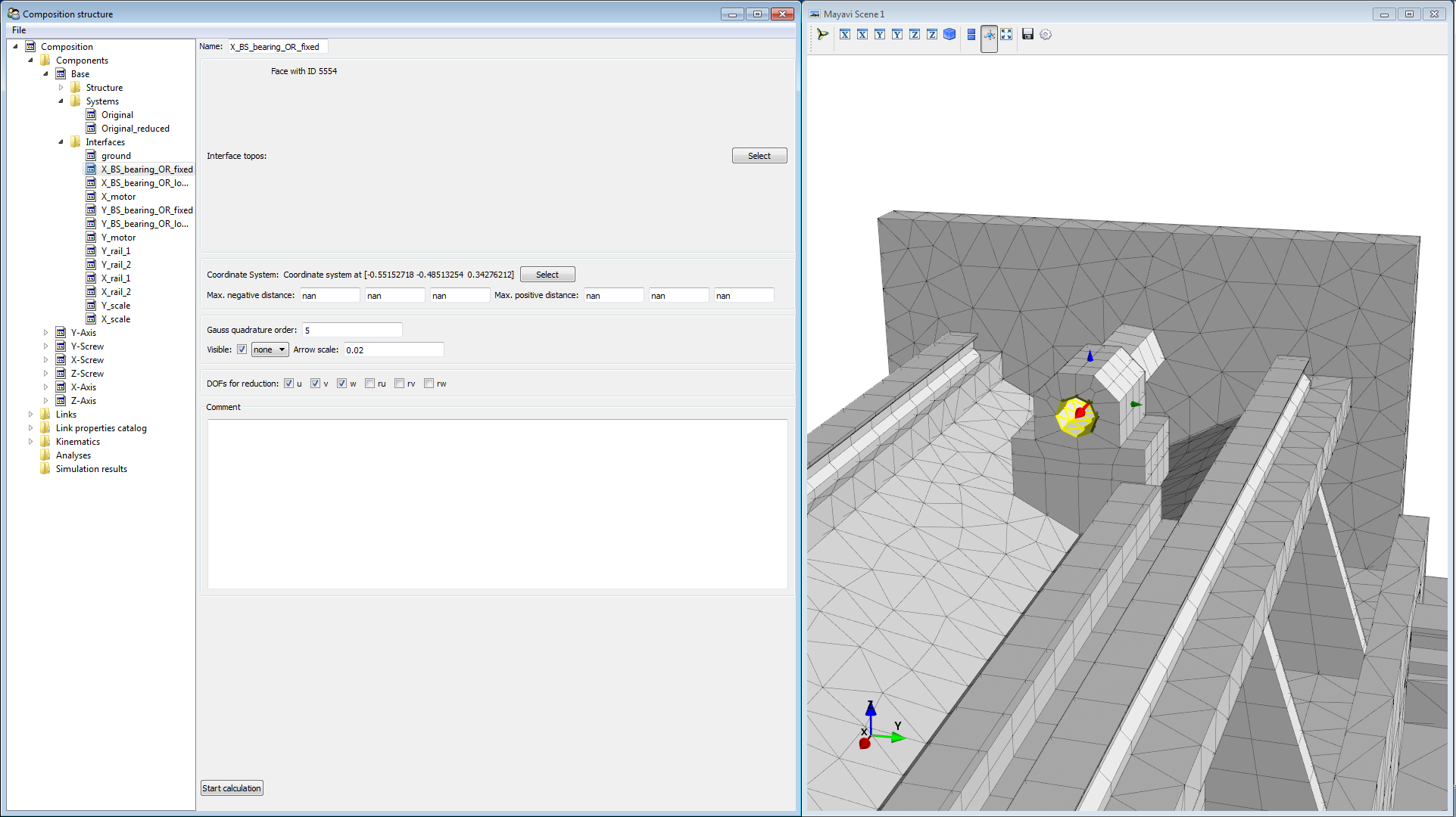
13. Create a 6dof interface for the outer ring of the fixed bearing of the X-axis ball screw. Define the coordinate system: u in x-direction, v in y-direction, w in z-direction. The fixed bearing transmits forces in u, v, w and has some friction in ru direction. Remove rv and rw from DOFs for reduction

    
    
    

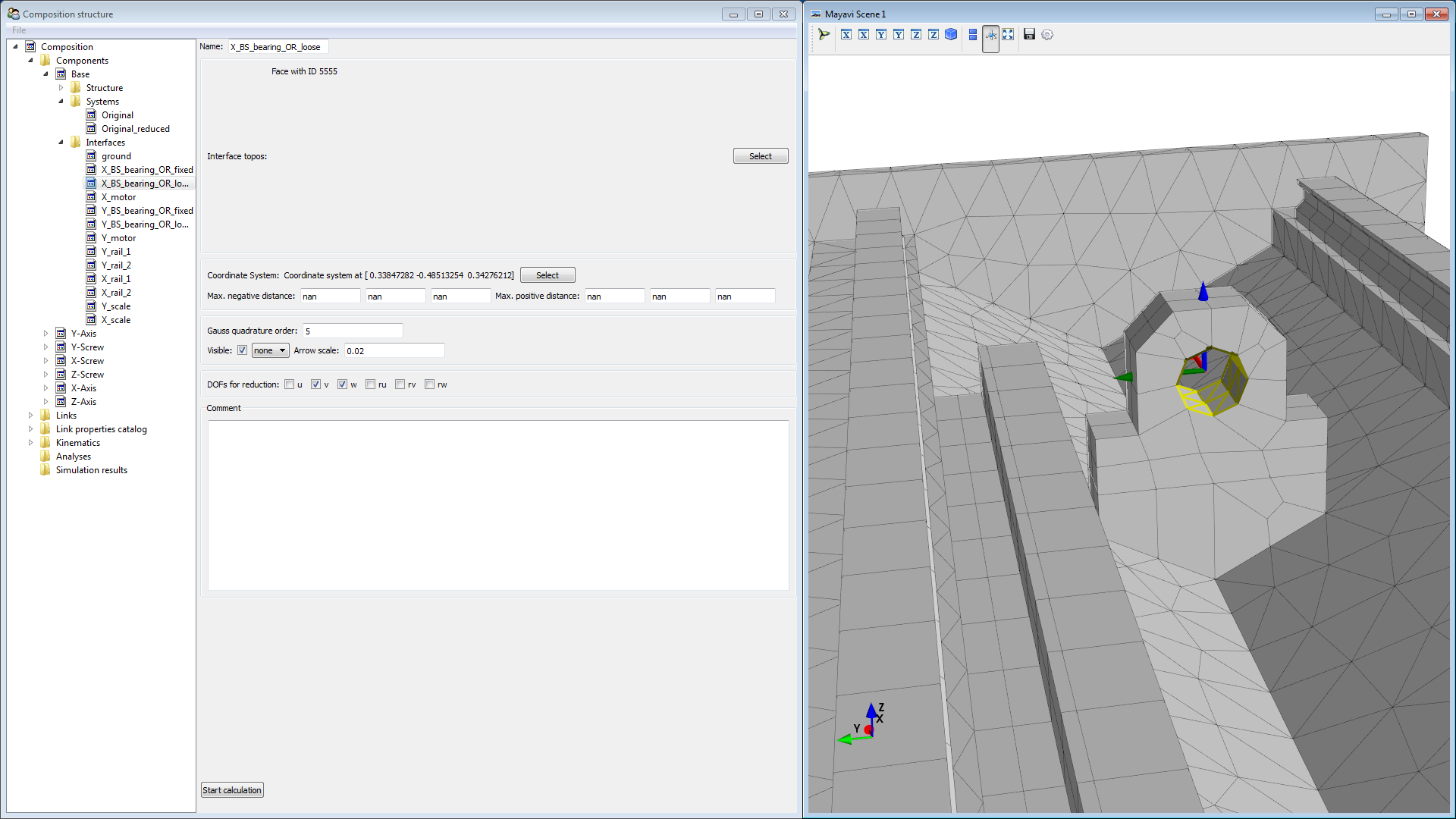
14. Create a 6dof interfaces for the outer ring of the loose bearing of the X-axis ball screw. Define the coordinate system: u in x-direction, v in y-direction, w in z-direction. Since the loose bearing applies no force in axial direction, remove u, rv, rw from DOFs for reduction

    
    
    

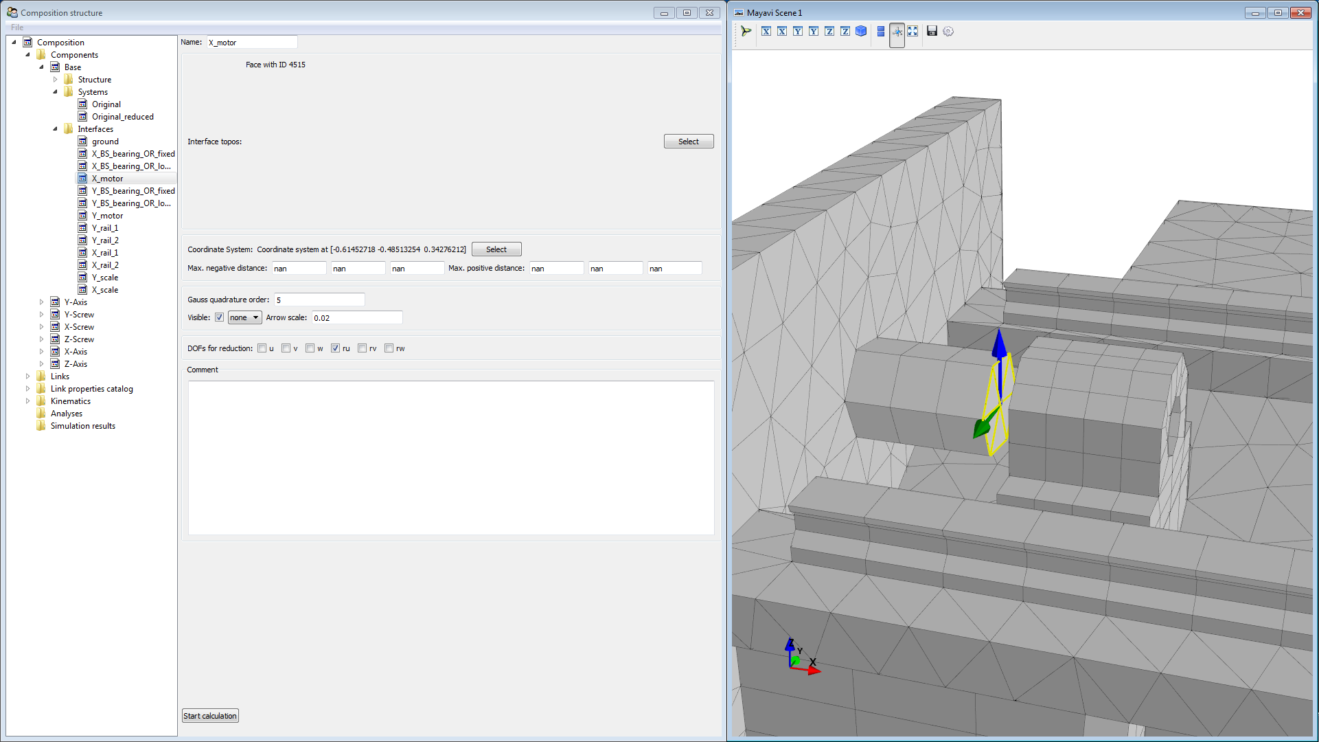
15. Create a 6dof interface for the reaction torque of the motor. The motor only applies torque in ru direction, thus we remove the other directions from DOFs for reduction

    
    
    

16. Create the interfaces for the Y-ball-screw bearings and the motor in the same way. Define the coordinate systems: axial(u) in y-direction, transversal (v) in negative x-direction, normal (w) in z-direction.

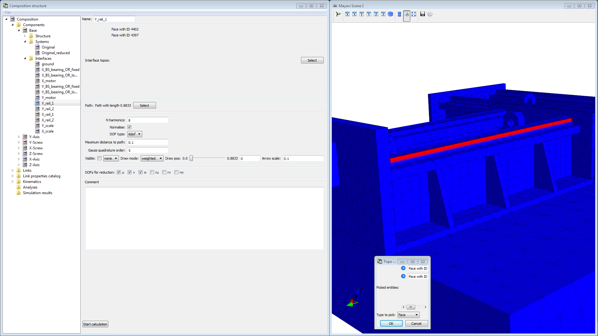
17. Next we will consider the rails. Since the carriages will move on the rails, we have to use moving interfaces for the rails. We start with the first rail of the Y-axis. Open the context menu for interfaces in the model tree, then select New Fourier Interface. Rename the new interface to Y_rail_1. Click Select in the interface topo box. Then select the faces for force transmission in the graphics window.

    
    
    

18. The next step is to define the movement path. Click Select in the Path box (1). Then Choose start topos (2). In the topo-picker box choose Vertex (3). Then select the vertices that mark the beginning of the faces we selected in the step before (4). Do not forget to select the vertices on the back side as well (4 in total)

    
    
    

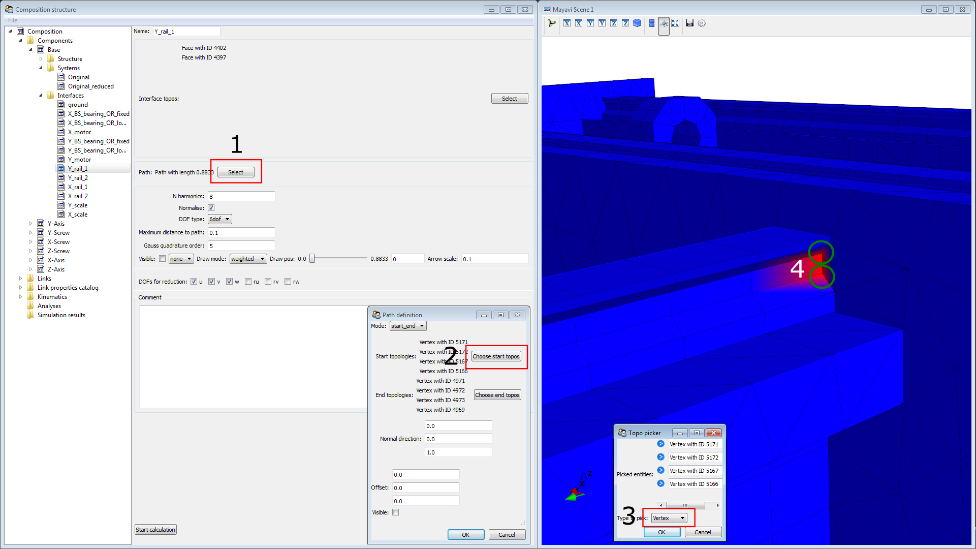
19. Choose end topos. Again select the 4 vertices. The normal direction is already correct. Click OK on the Path definition Box

    
    
    

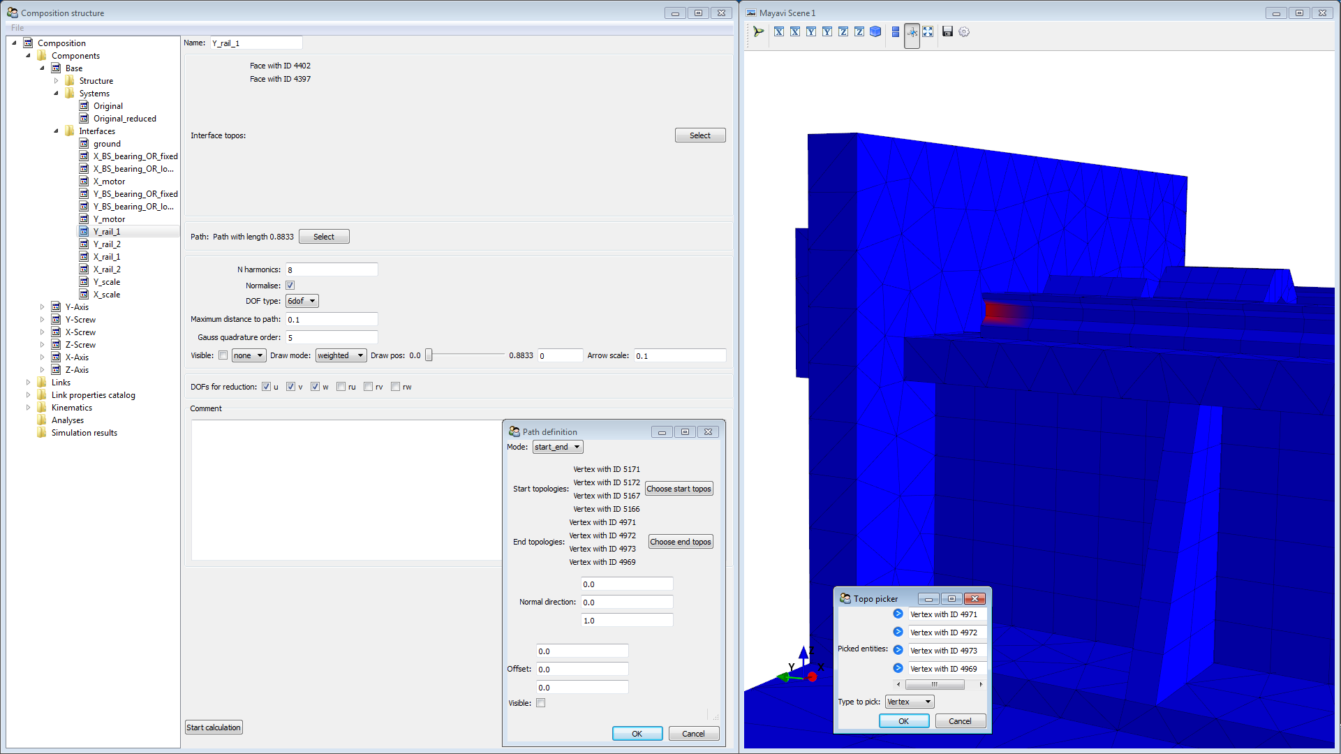
20. Enter a value for N harmonics. This setting “divides” the path into smaller pieces. One piece should approximately have the length of the carriage. Thus we enter 8. The other setting we leave on default. Select u, v, w in DOFs for reduction. Then click Start calculation. This will take a few minutes.

    
    
    

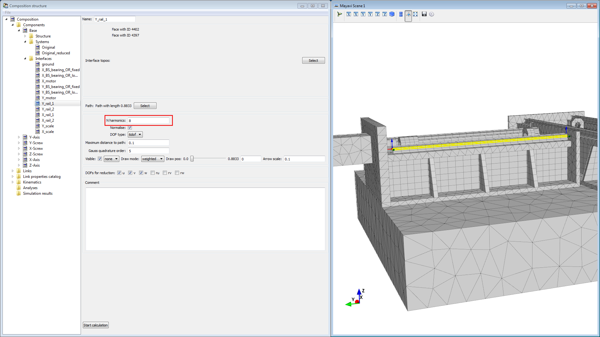
21. Repeat for the other Y-rail. Then for the X-rails. Since the X-rails are longer, use N harmonics of 10.

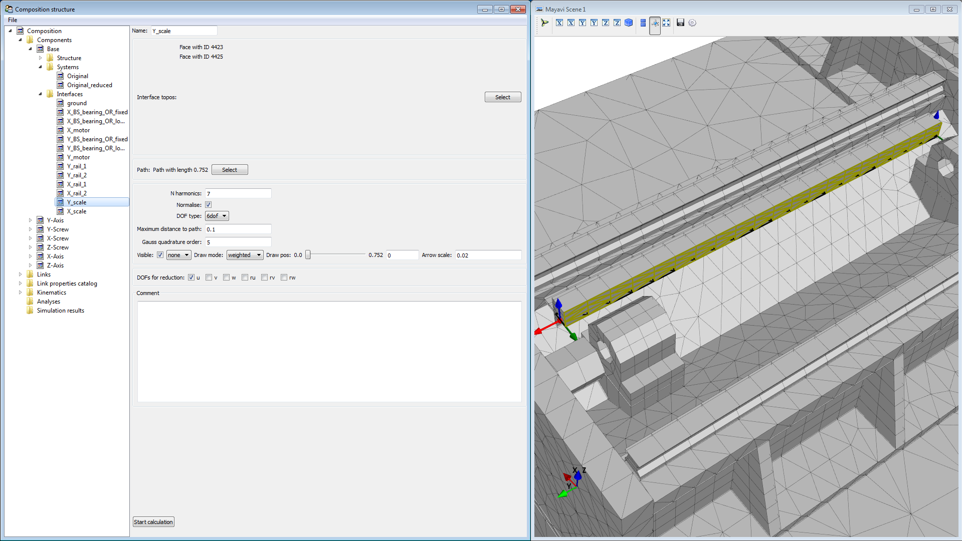
22. Define a Fourier Interface for the measuring scale of the Y-axis. Moving interfaces require the selection of faces with an extent in both directions orthogonal to the path. Therefore, in this case, the bottom and side face of the scale geometry are selected. A number of harmonics of 5 is appropriate.

    
    
    

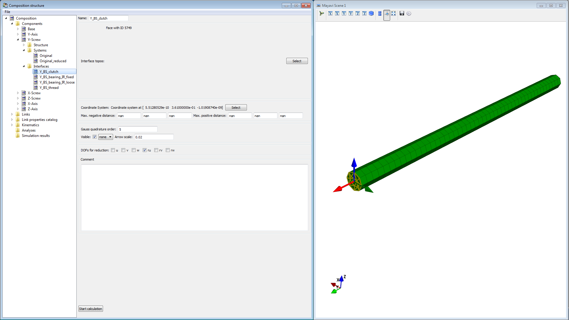
23. Next we will define the interfaces for the ball screws. Hide the Base component and show the Y-Screw component. Define a 6dof interface on the end face next to the motor. Name it Y_BS_clutch. Define the coordinate System in the same orientation as for the other Y interfaces (axial in Y-direction, transversal in negative X-direction, normal in Z-direction). The clutch only transmits torque in ru direction, thus remove the other directions from DOFs for reduction.

    
    
    

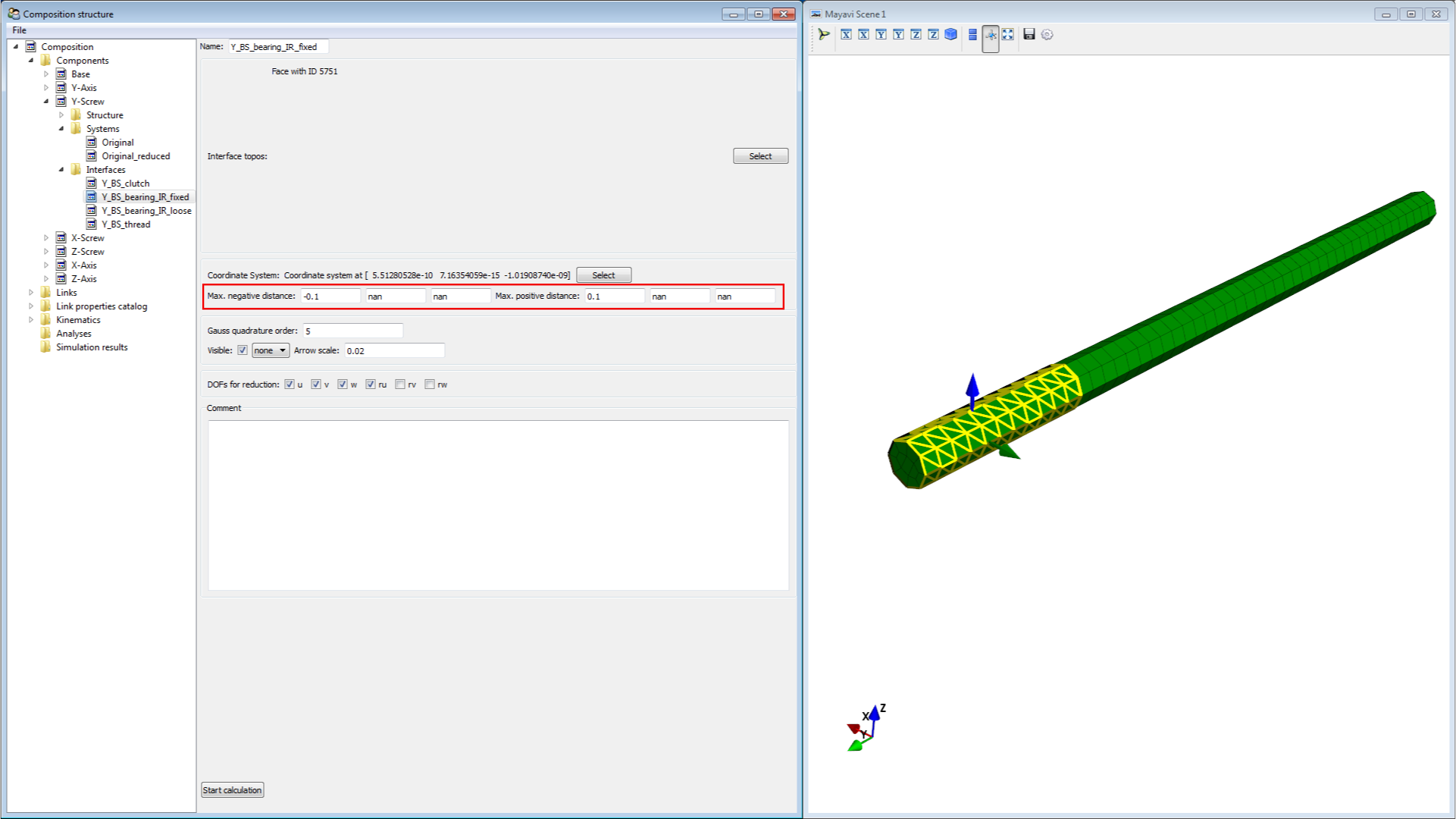
24. Create a interface for the fixed bearing of the Y-ball-screw. Create a new 6dof interface, name it Y_BS_bearing_IR_fixed (IR for inner ring). Select the shell of the screw. Define the coordinate system as for the other Y components. The force that is applied to the bearing is not evenly distributed over the whole shell, thus we limit the area by entering -0.1 for Max. negative distance and 0.1 for Max. positive distance. You will notice, that the coordinate system is in the middle of the screw and not where the bearing is located. We will fix this later when defining links. The bearing only transmits forces in u,v,w and friction in ru direction, thus deselect the others.

    
    
    

25. Create a 6dof interface for the loose bearing with the name Y_BS_bearing_IR_loose. Again set Max. negative distance to -0.1 and Max. positive distance to 0.1. Only select v,w in DOFs for reduction (the loose bearing transmits no force in axial direction).

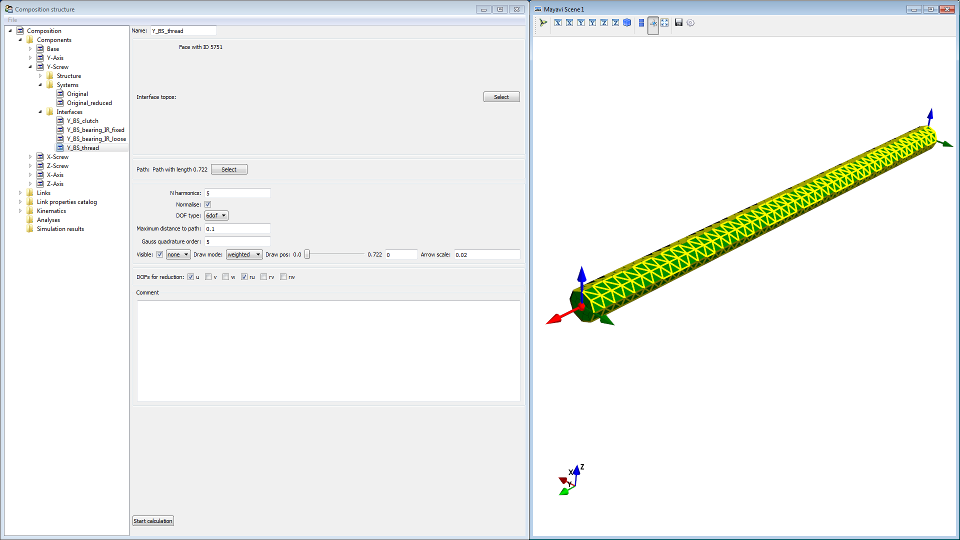
26. Next we create a moving interface (Fourier interface) for the connection between ball screw and nut. Select the shell of the ball screw for Interface topos. Then define the path by selecting the end faces of the screw. N harmonics of 5 is appropriate. The ball screw only transmits force in u direction and torque around u, i.e. ru direction, remove the others.

    
    
    

27. Define all remaining interfaces. When done you should have the following interfaces for each component:

    • Base

      • Ground (1x 6dof)

        • ground

      • Ball screw bearings outer rings X, Y (4x 6dof)

        • X_BS_bearing_OR_fixed

        • X_BS_bearing_OR_loose

        • Y_BS_bearing_OR_fixed

        • Y_BS_bearing_OR_loose

      • Rails X, Y (4x Fourier)

        • X_rail_1

        • X_rail_2

        • Y_rail_1

        • Y_rail_2

      • Motors X, Y (2x 6dof)

        • X_motor (to get positive movement of the axis for positive rotation of the screw, this interface has to defined inverse. define u in negative X direction)

        • Y_motor

      • Linear scales(2x Fourier)

        • X_scale

        • Y_scale

    • X-Axis

      • Carriages X (4x 6dof)

        • X_carriage_11

        • X_carriage_12

        • X_carriage_21

        • X_carriage_22

      • Ball screw nut X (1x 6dof)

        • X_BS_nut

      • Ball screw bearings outer rings Z (2x 6dof)

        • Z_BS_bearing_OR_fixed

        • Z_BS_bearing_OR_loose

      • Rails Z (2x Fourier)

        • Z_rail_1

        • Z_rail_2

      • Motor Z

        • Z_motor (to get positive movement of the axis for positive rotation of the screw, this interface has to defined inverse. define u in negative Z direction)

      • Encoders(1x 6dof)

        • X_encoder

      • Linear scales(1x Fourier)

        • Z_scale

    • Y-Axis

      • Carriages Y (4x 6dof)

        • Y_carriage_11

        • Y_carriage_12

        • Y_carriage_21

        • Y_carriage_22

      • Ball screw nut Y (1x 6dof)

        • Y_BS_nut

      • Workpiece

        • workpiece (use global coordinate system)

      • Encoders 1x 6dof)

        • Y_encoder

    • Z-Axis

      • Carriages Z (4x 6dof)

        • Z_carriage_11

        • Z_carriage_12

        • Z_carriage_21

        • Z_carriage_22

      • Ball screw nut Z (1x 6dof)

        • Z_BS_nut

      • TCP (1x 6dof)

        • TCP (use global coordinate system)

      • Encoder (1x 6dof)

        • Z_encoder

    • X-Screw

      • Clutch

        • X_BS_clutch (to get positive movement of the axis for positive rotation of the screw, this interface has to defined inverse. define u in negative X direction)

      • Ball screw bearings inner rings X (2x 6dof)

        • X_BS_bearing_IR_fixed

        • X_BS_bearing_IR_loose

      • Ball screw thread X (1x Fourier)

        • X_BS_thread

    • Y-Screw

      • Clutch

        • Y_BS_clutch

      • Ball screw bearings inner rings Y (2x 6dof)

        • Y_BS_bearing_IR_fixed

        • Y_BS_bearing_IR_loose

      • Ball screw thread Y (1x Fourier)

        • Y_BS_thread

    • Z-Screw

      • Clutch

        • Z_BS_clutch (to get positive movement of the axis for positive rotation of the screw, this interface has to defined inverse. define u in negative Z direction)

      • Ball screw bearings inner rings Z (2x 6dof)

        • Z_BS_bearing_IR_fixed

        • Z_BS_bearing_IR_loose

      • Ball screw thread Z (1x Fourier)

        • Z_BS_thread

Link properties

After having defined all required interfaces, we define the properties of the links between them.

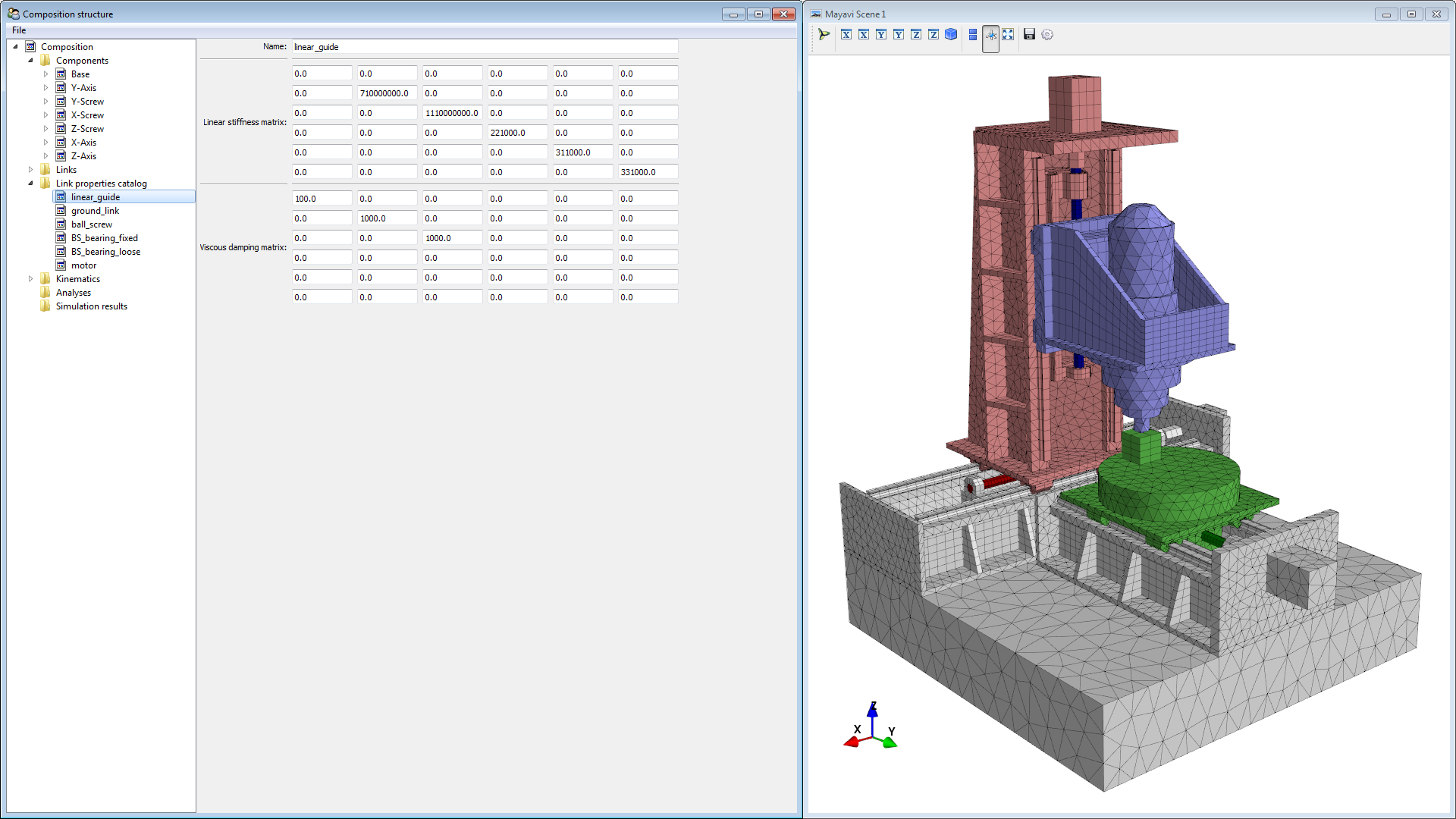
1. Right-click on link properties catalog and select New linear link property, name it linear_guide. Enter the rigidities for the linear guide on the diagonal of the matrix. For this machine we use the following values:

   • Stiffness: (0, 710e6, 1110e6, 221e3, 311e3, 331e3) [N/m respectively Nm/rad]

   • Damping (100, 1000, 1000, 0, 0, 0) [Ns/m respectively Nms/rad]

   
   
   
   
   

2. Create a new linear link property for the base to ground connection. Name it ground_link and add the following stiffness.

   • Stiffness: (1e9, 1e9, 1e9, 1e9, 1e9, 1e9) [N/m respectively Nm/rad]

   • Damping (1000, 1000, 1000, 1000, 1000, 1000) [Ns/m respectively Nms/rad]

   
   

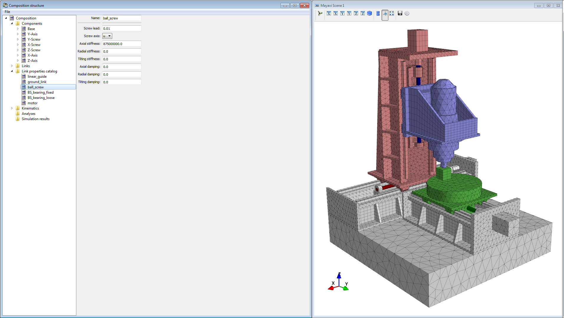
3. Create a link property for the ball screw links. Right-click on Link properties catalog and select New linear screw link. Name it ball_screw. Enter the ball screw properties:

   • Screw lead: 0.01

   • Screw axis: u

   • Axial stiffness: 875e6

   
   
   
   
   

4. Create a linear link property for the fixed ball screw bearing. Name it BS_bearing_fixed

   • Stiffness: (990e6, 165e6, 165e6, 0, 0, 0) [N/m respectively Nm/rad]

   • Damping (750, 500, 500, 0.05, 0, 0) [Ns/m respectively Nms/rad]

   
   

5. Create a linear link property for the loose ball screw bearing. Name it BS_bearing_loose

   • Stiffness: (0, 165e6, 165e6, 0, 0, 0) [N/m respectively Nm/rad]

   • Damping (0, 500, 500, 0.05, 0, 0) [Ns/m respectively Nms/rad]

   
   

Links

With the interfaces and the link properties we now create the links, i.e. couplings between two interfaces or one interface and ground.

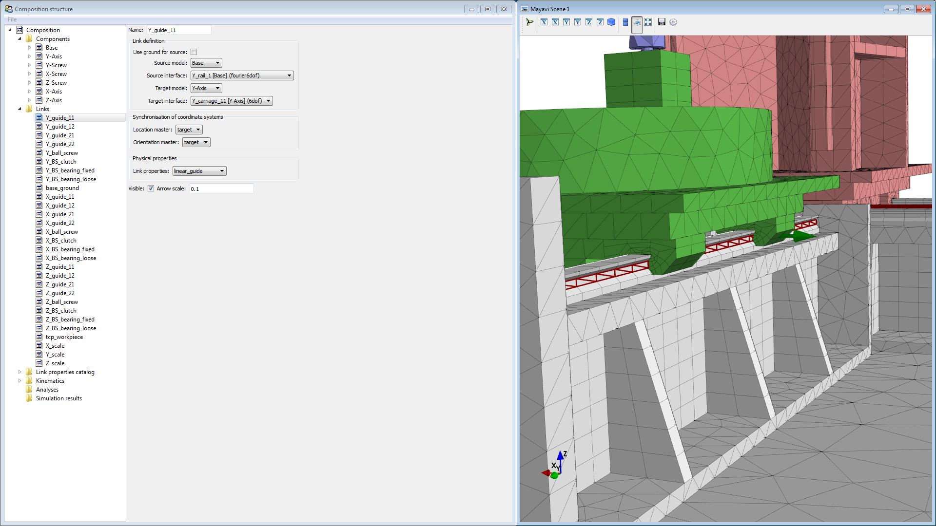
1. We Start with the Y-axis. Right-click on Links in the tree and select New link. Name it Y_guide_11

   • Source model: Base

   • Source interface: Y_rail_1

   • Target model: Y-Axis

   • Target interface: Y_carriage_11

   • Location master: target (this defines that the location of action of the link is at the position of the target interface. This is necessary for the correct function of moving interfaces)

   • Orientation master: target

   • Link properties: linear_guide

   
   
   

2. Repeat for the other 3 carriages.

3. Create a link for the connection of the Y-ball-screw to the nut. Name it Y_ball_screw

   • Source model: Y-screw

   • Source interface: Y_BS_thread

   • Target model: Y-Axis

   • Target interface: Y_BS_nut

   • Location master: target

   • Orientation master: target

   • Link properties: ball_screw

4. Create a link for the Y clutch (Y_BS_clutch)

   • Source model: Base

   • Source interface: Y_motor

   • Target model: Y-Screw

   • Target interface: Y_BS_clutch

   • Location master: target

   • Move slave interface: not ticked (Move slave interface defines if the coordinate system of the slave interface is moved or if only a virtual cantilever is applied to this interface)

   • Orientation master: target

   • Link properties: None (we will use this interface to apply torque)

5. Create a link for the fixed bearing of the Y-ball-screw (Y_BS_bearing_fixed)

   • Source model: Base

   • Source interface: Y_BS_bearing_OR_fixed

   • Target model: Y-Screw

   • Target interface: Y_BS_bearing_IR_fixed

   • Location master: source

   • Move slave interface: ticked (the target coordinate system is in the middle of the screw and needs to be moved to the place where the bearing is)

   • Orientation master: source

   • Link properties: BS_bearing_fixed

6. Create a link for the loose bearing of the Y-ball-screw (Y_BS_bearing_loose)

   • Source model: Base

   • Source interface: Y_BS_bearing_OR_loose

   • Target model: Y-Screw

   • Target interface: Y_BS_bearing_IR_loose

   • Location master: source

   • Orientation master: source

   • Link properties: BS_bearing_loose

7. Create a link for the measuring scale (Y_scale)

   • Source model: Base

   • Source interface: Y_scale

   • Target model: Y-Axis

   • Target interface: Y_encoder

   • Location master: target

   • Orientation master: target

   • Link properties: None

8. Create a link for the base - ground connection (base_ground)

   • Use ground for source: tick

   • Target model: Base

   • Target interface: ground

   • Link properties: ground_link

9. Define the links for the X and Z axes following the same procedure. Also add a link with workpiece as source and TCP as target (name it tcp_workpiece)

Model order reduction

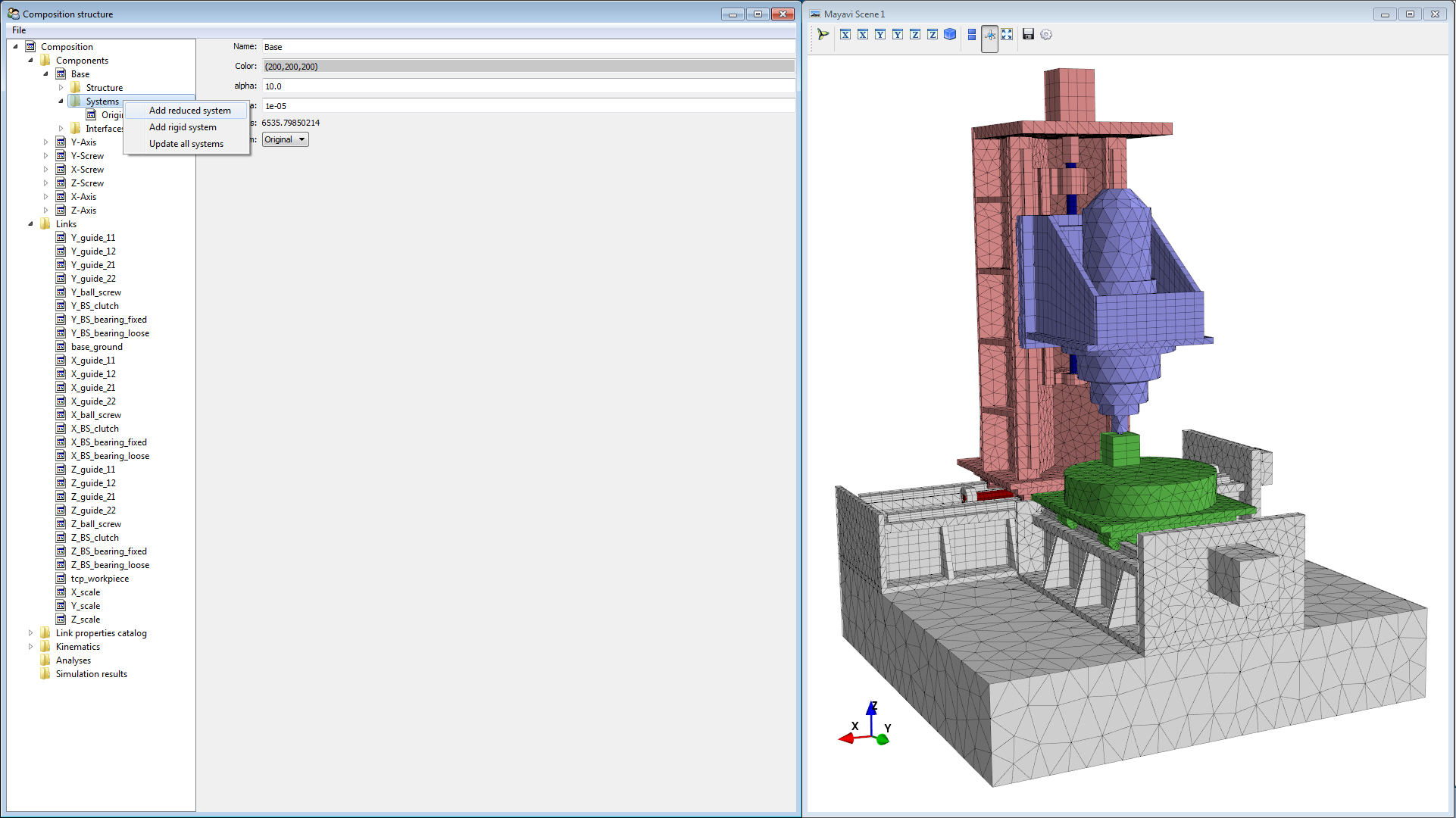
1. Create a new reduced system for the base component. Expand Base then right-click on Systems and select Add reduced system.

   
   
   

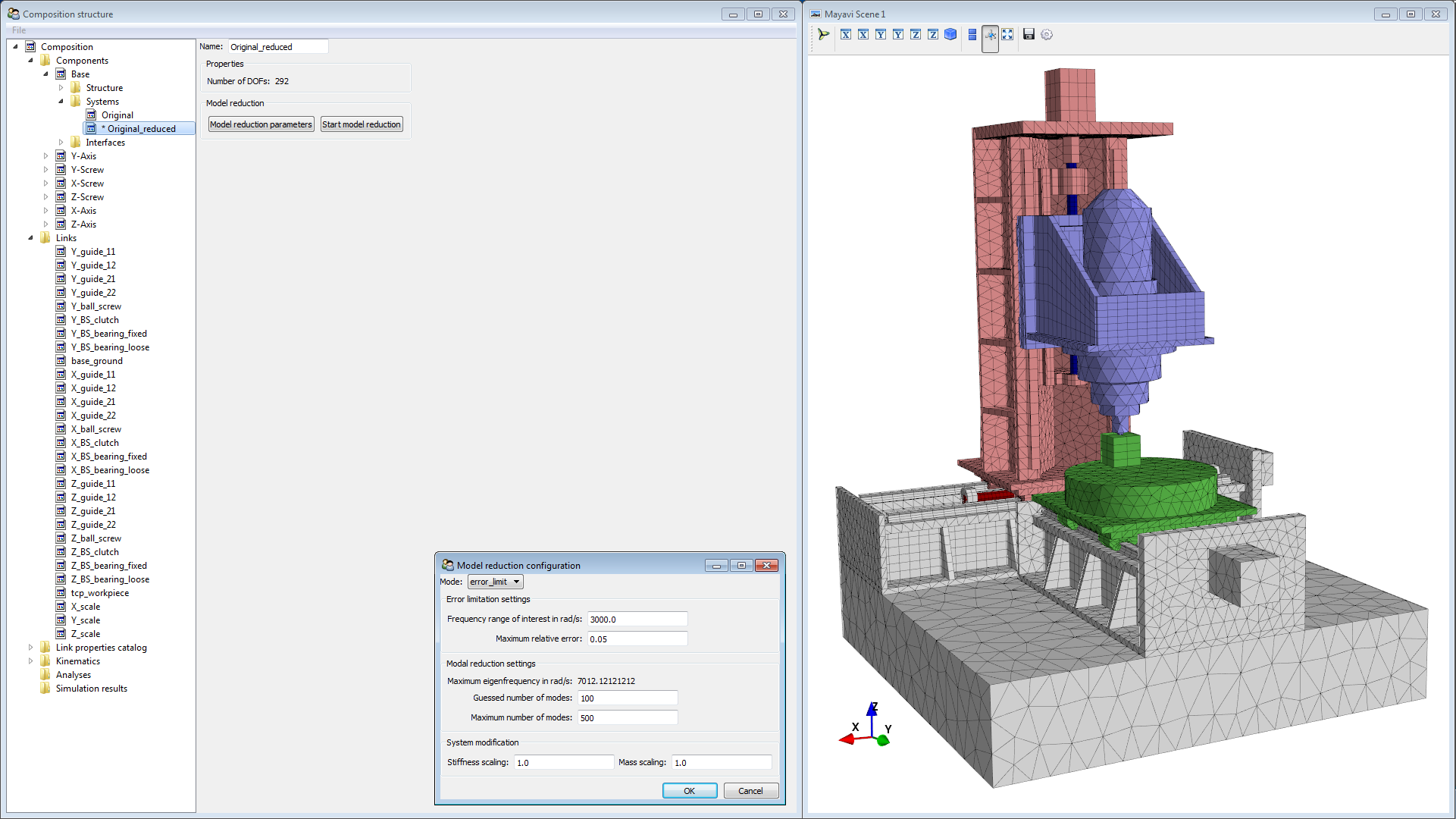
2. Click on the newly created system called Original_reduced and then press the Model reduction parameters button. Modify the properties as follows and complete with OK.

   • Mode: error_limit

   • Error limitation settings

     • Frequency range of interest in rad/s: 3000 (This equals approximately 500Hz, which is about 10 times the controller bandwidth)

     • Maximum relative error: 0.05 (Maximum magnitude error of 5%)

   • Modal reduction settings

     • Maximum eigenfrequency in rad/s: read-only (This is the maximum eigenfrequency considered for modal reduction)

     • Guessed number of modes: 200 (How many modes are estimated below the maximum eigenfrequency)

     • Maximum number of modes: 500 (The limit number of modes to calculate before stopping if the desired frequency is not reached)

   • System modification

     • Stiffness scaling: 1.0

     • Mass scaling: 1.0

   
   
   
   
   

3. Click on Start model reduction. This updates the interface definitions if necessary (if there are asterisk prefixes) and invokes the model reduction routine afterwards. This takes some time. Look at the console for status information. When the reduction is completed, the asterisk in the system name disappears. As soon as an interface is added or modified, the system gets a new asterisk and should then be reduced again.

4. Reduce all the other components in the same way. Don’t forget to save the composition afterwards.

Kinematics

In order enable changing of initial positions for simulation, we need to define the machine’s kinematics, i.e. the rules how the components move with the axes.

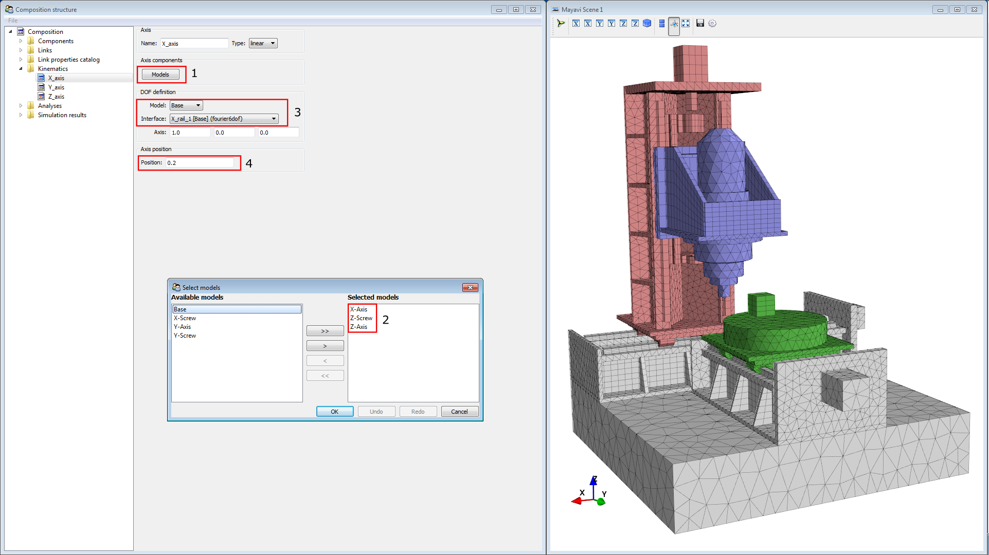
1. Right-click on Kinematics in the tree, select Add axis. Name it to X_axis, click on Models (1) then select the X-Axis, the Z-Axis and the Z-Screw (2). In the DOF-definition box select X_rail_1 as interface (3). To check if it works correctly enter 0.2 in the Position field (4) to move the axis.

   
   
   

2. Add the Y- and Z-axis in the following way.

   • Y_axis

     • Axis components: Y-Axis

     • Model: Base

     • Interface: Y_rail_1

     • Axis: 1.0 ; 0 ; 0

   • Z_axis

     • Axis components: Z-Axis

     • Model: X-Axis

     • Interface: Z_rail_1

     • Axis: 1.0 ; 0 ; 0

Analyses

At the moment, following analyses are directly applicable from the MORe GUI:

• Modal analysis

• Frequency response analysis

• Static analysis

• Spatial static analysis

• Stiffness analysis

Modal Analysis

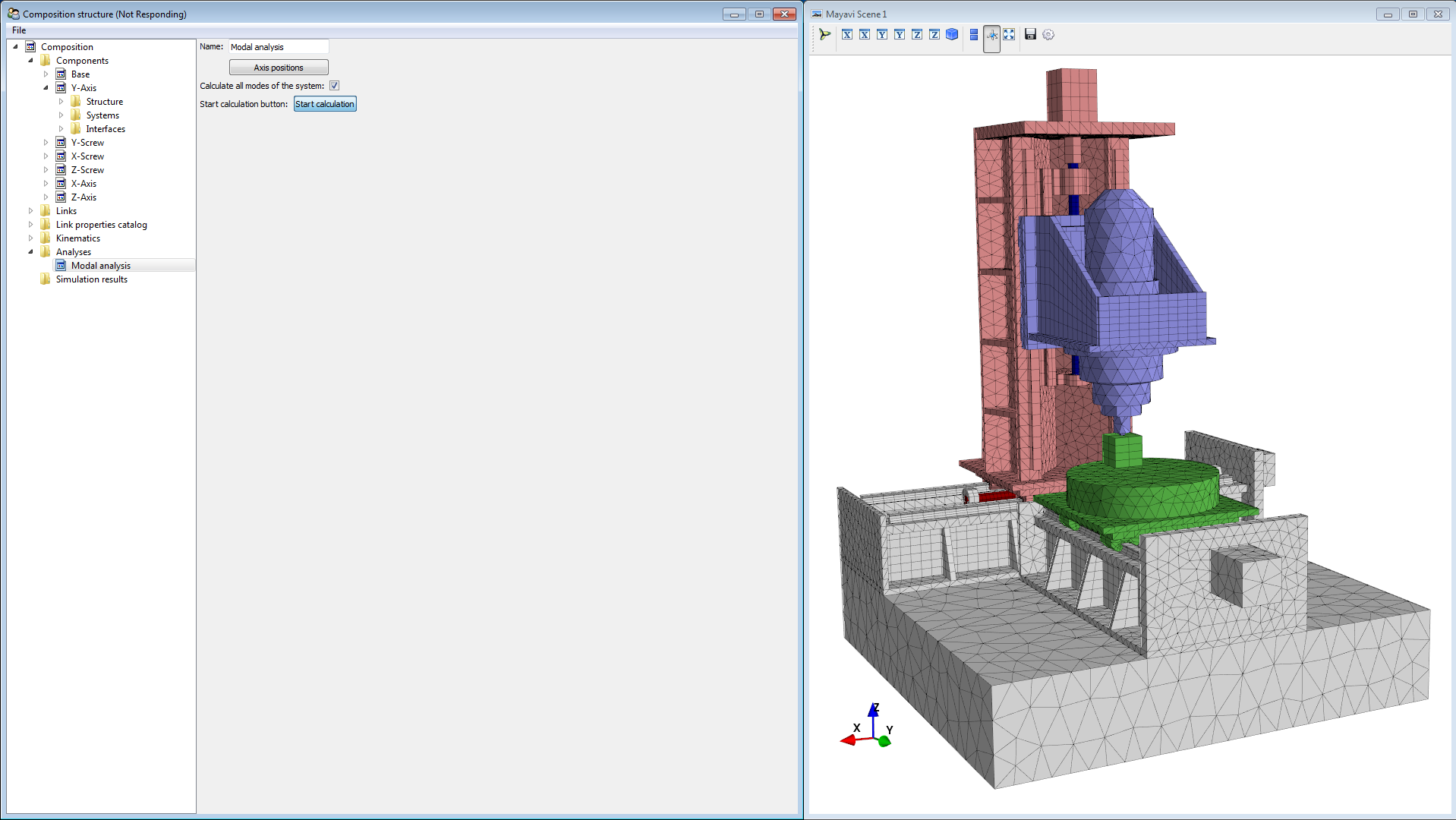
In order to check if all interfaces and links are defined correctly we create a modal analysis.

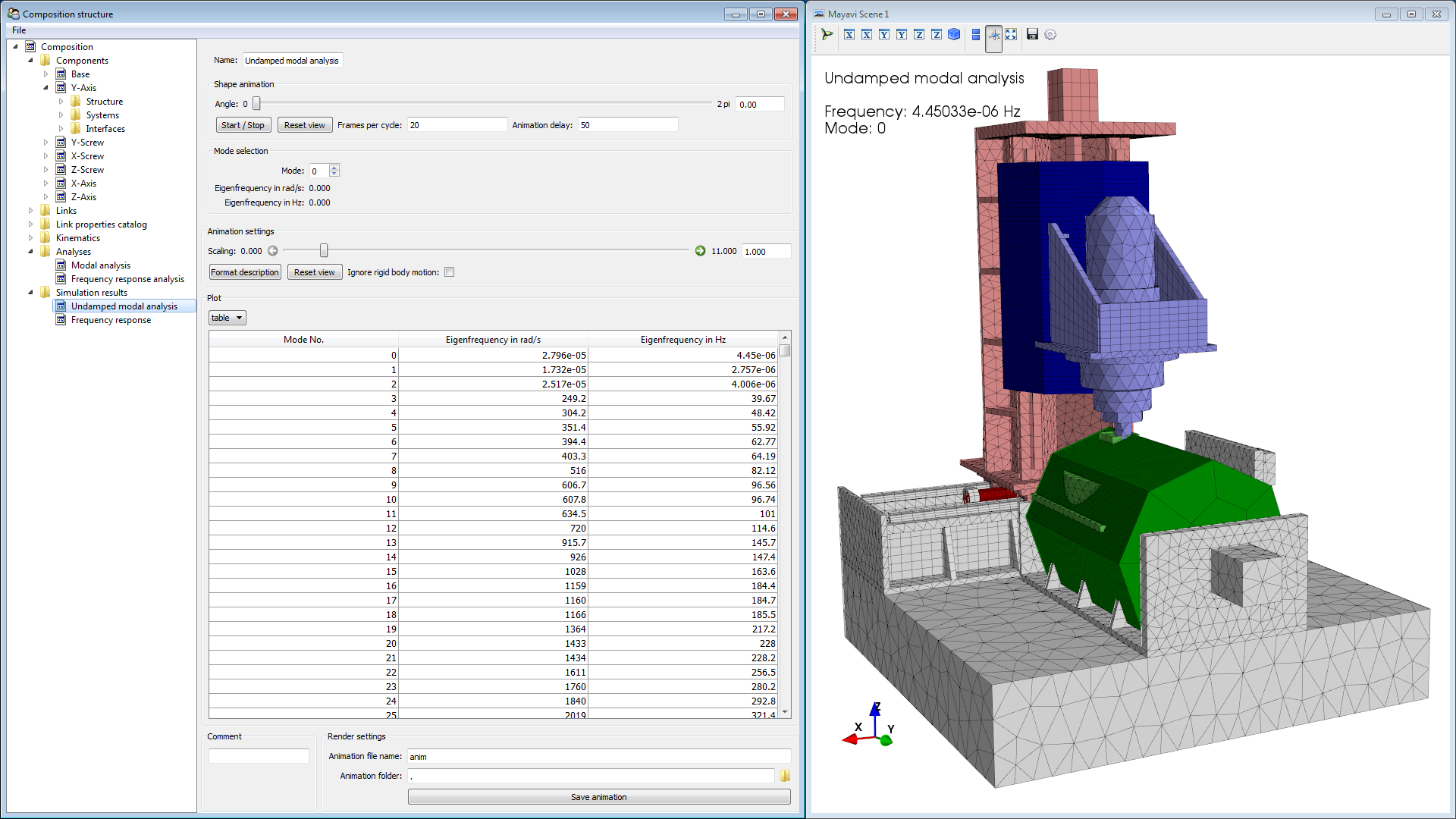
1. Right-click on Analyses in the tree and select Add modal analysis. Tick Calculate all modes of the system , then click Start calculation. Under Simulation results in the tree, an Undamped modal analysis appears. Click on it to show the analysis results. Start the animation and go through the modes of the system by increasing the mode number (click into the box and scroll with the mouse wheel). Now check if you got exactly 3 rigid body modes for the 3 axes of the machine (frequency close to zero). The rotation of the ball-screws looks unnatural when super-elevated, so you might want to hide them. Then check the modes for errors in the links or interfaces (wrong movements).

   
   
   
   
   
   

Frequency Response Analysis

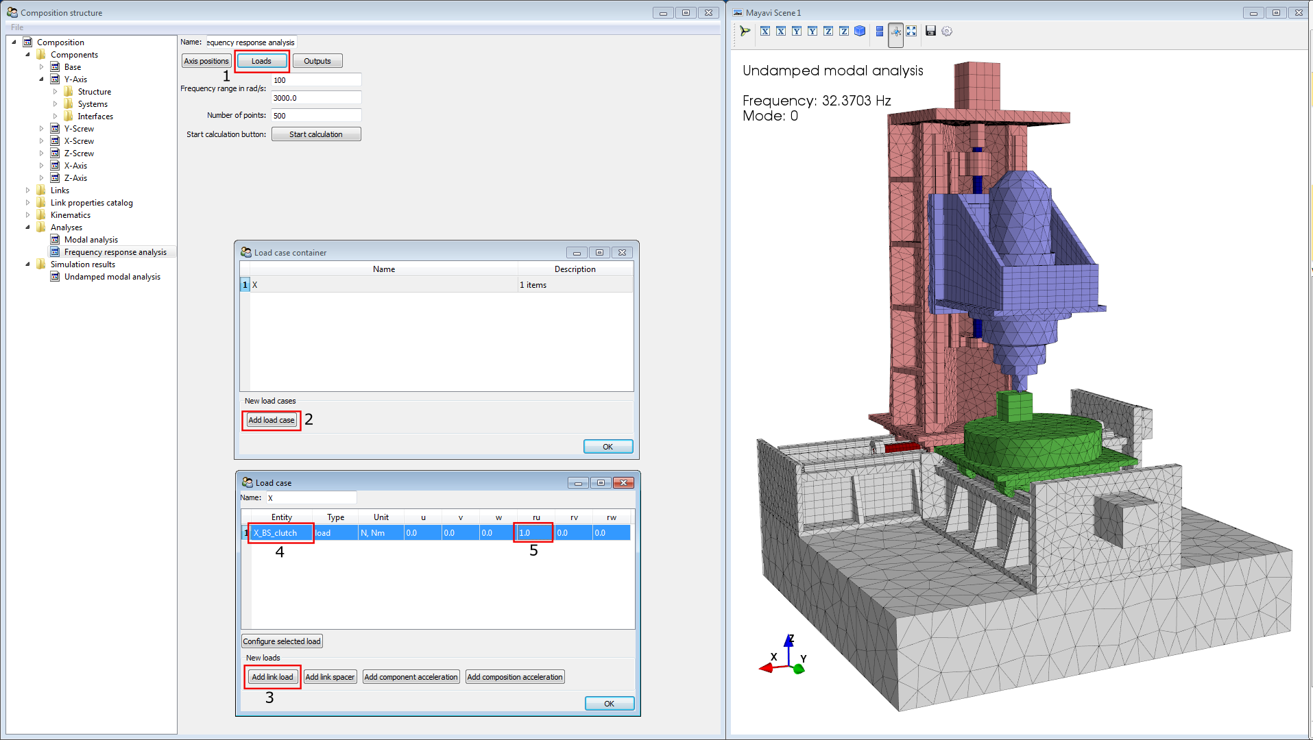
1. Right-click on Analyses and select Add frequency response analysis. Click Loads (1) and then Add load case (2) to add a new load case. Rename the load case to X. Select the newly created row and press Ctrl+K to evoke the configuration window for the particular load case. Click on Add link load (3) and select the link X_BS_clutch (4), insert the value 1 for the ru direction (5). This means we apply torque (scaled by 1) to the X_BS_clutch in ru direction (rotate the screw).

   
   
   

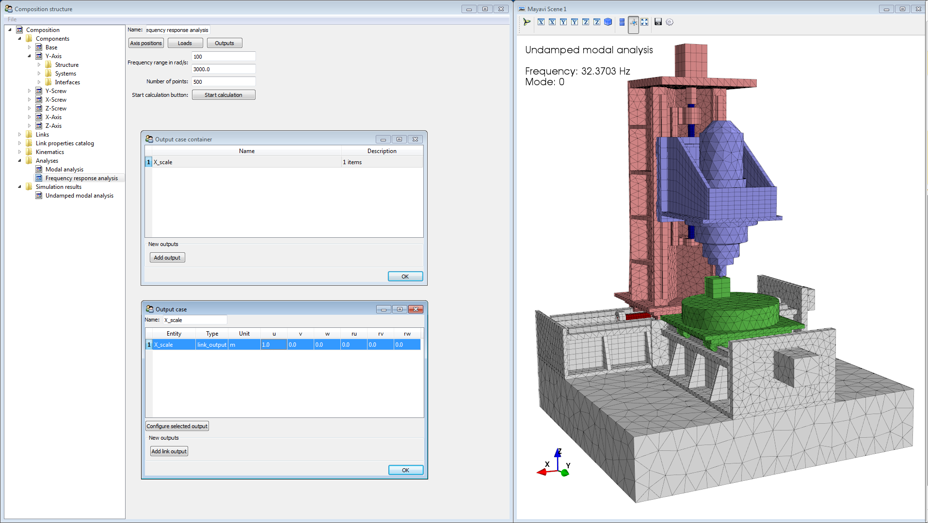
2. Click on Outputs and define an output for the X_scale link in u-direction. Select a frequency range from 100 to 3000 rad/s, then start the calculation.

   
   
   

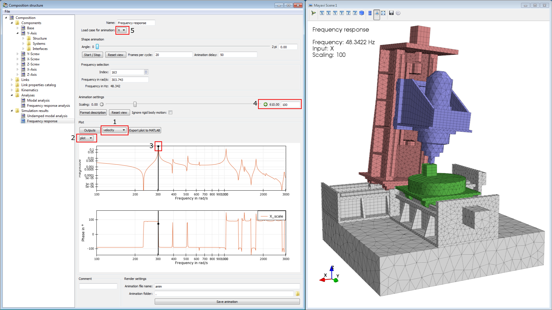
3. The results will again appear under Simulation results. Select velocity (1) as this gives the velocity open-loop Bode diagram. Switch the table view to a Bode plot view (2). Now you can drag the black point on the plot (3) to the interesting areas (resonance and antiresonance frequencies). Start the animation and use (4) to adjust the scaling. If multiple load cases have been defined, use (5) to select the desired one.

   
   
   

MATLAB/Simulink

For more advanced analyses and to design a controller for the machine you can use the MORe model with MATLAB and Simulink.

1. Create a new MATLAB script file and enter the code for the import of a composition (project) file. The comp object then contains all necessary information about the model.

   %% Load MORe composition
   comp = Composition(); % create composition object
   % define the path to the composition you saved from MORe
   comp_filepath = '..\MORe_comp';
   comp_filename = '20171013_rekowema.comp';
   comp.import(fullfile(comp_filepath,comp_filename));
   

2. Open the MORe simulink library by entering open('more_library') to the command window.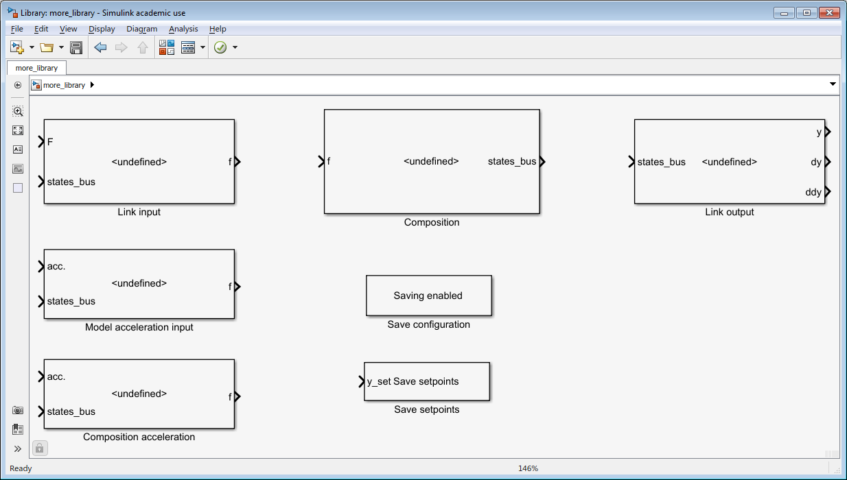

   
   
   

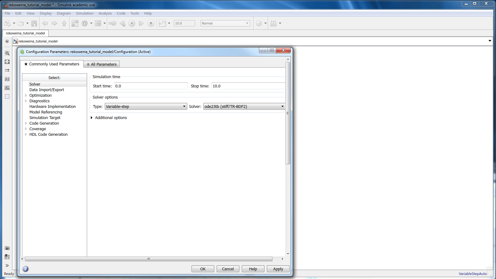
3. Create a new blank Simulink model. Save it as rekowema_tutorial_model. Open Model configuration parameters and change the solver to ode23tb.

   
   
   

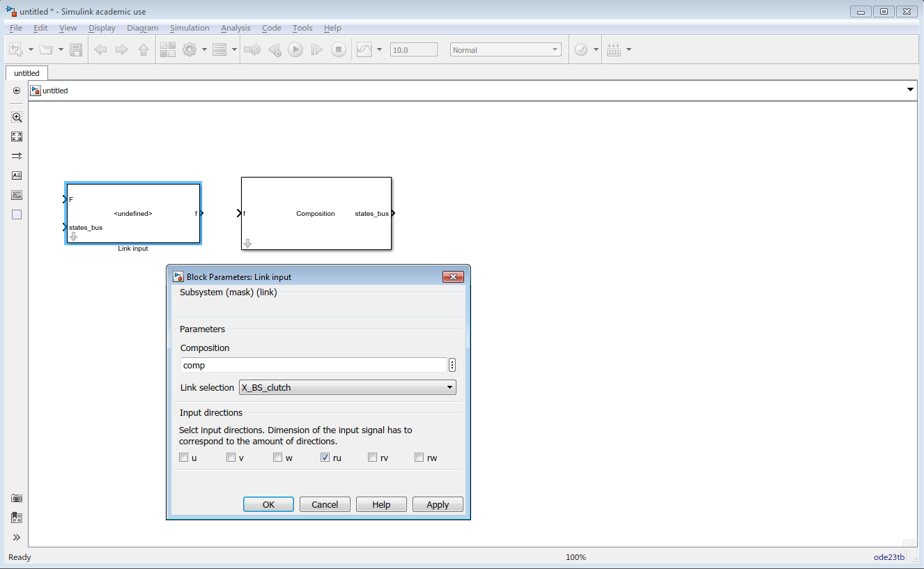
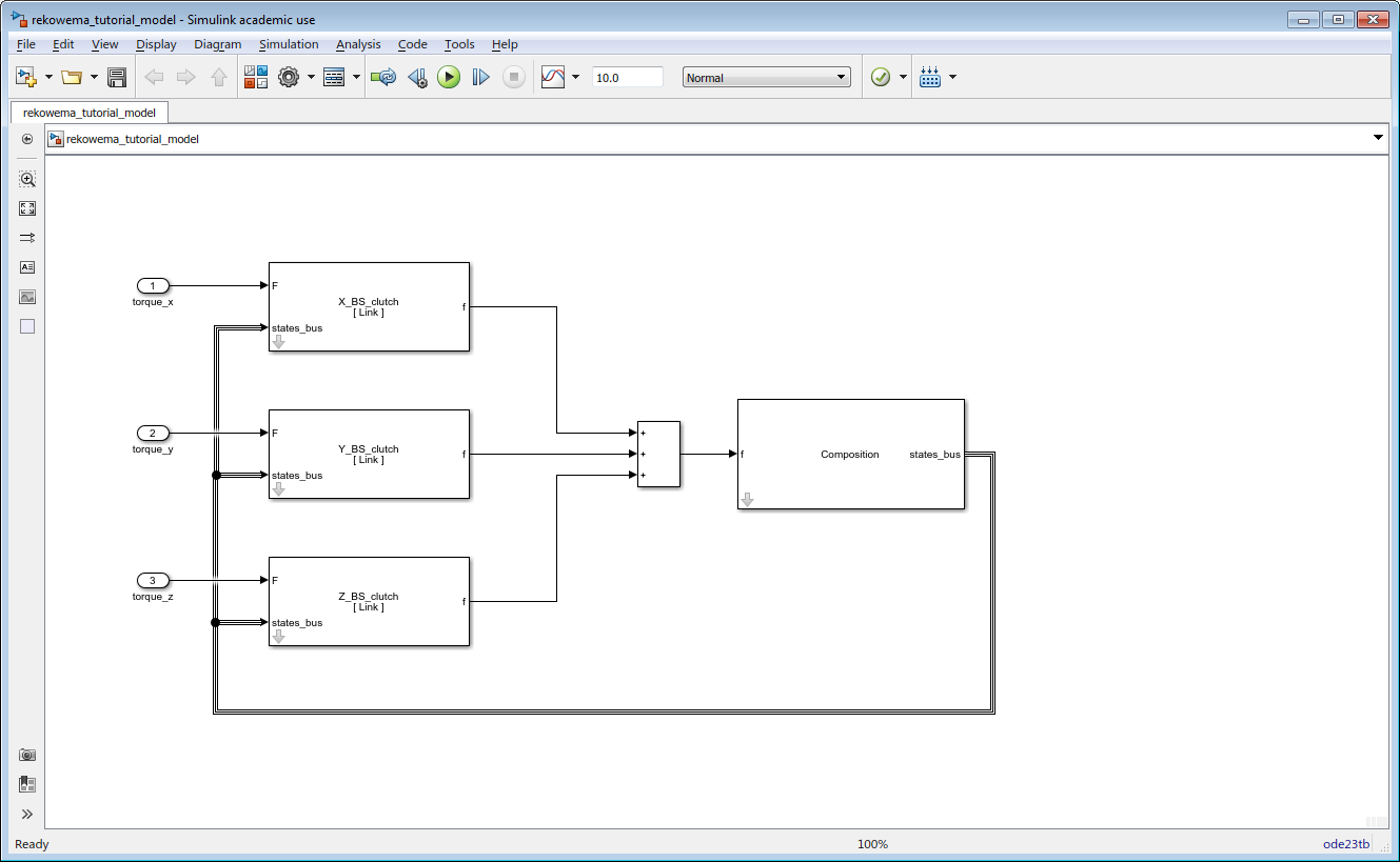
4. Drag a Composition block from the more library to the new model. This block contains the model that was loaded to the workspace (as comp). Next, we add an input for the torque to the X-axis’ ball screw. Drag a Link input block to your model. Double-click it, then select X_BS_clutch which is the link we created to apply torque to the ball screw. Select the ru-direction only. The Link input block has 3 ports

   • F: is the input for the force applied to the link as vector with as many elements as selected directions (u, v, w, ru, rv, rw). In this case, it is a scalare torque.

   • states_bus: needs to be connected to the states bus port of the Composition block.

   • f: force output for each state of the model that connects to the f port of the Composition block.

   
   
   
   
   

5. Add Link input blocks for the Y- and the Z-axis. For the force input add Simulink/Sources/In blocks. Rename the In blocks to torque_x, torque_y and torque_z. Then add the connections between the blocks.

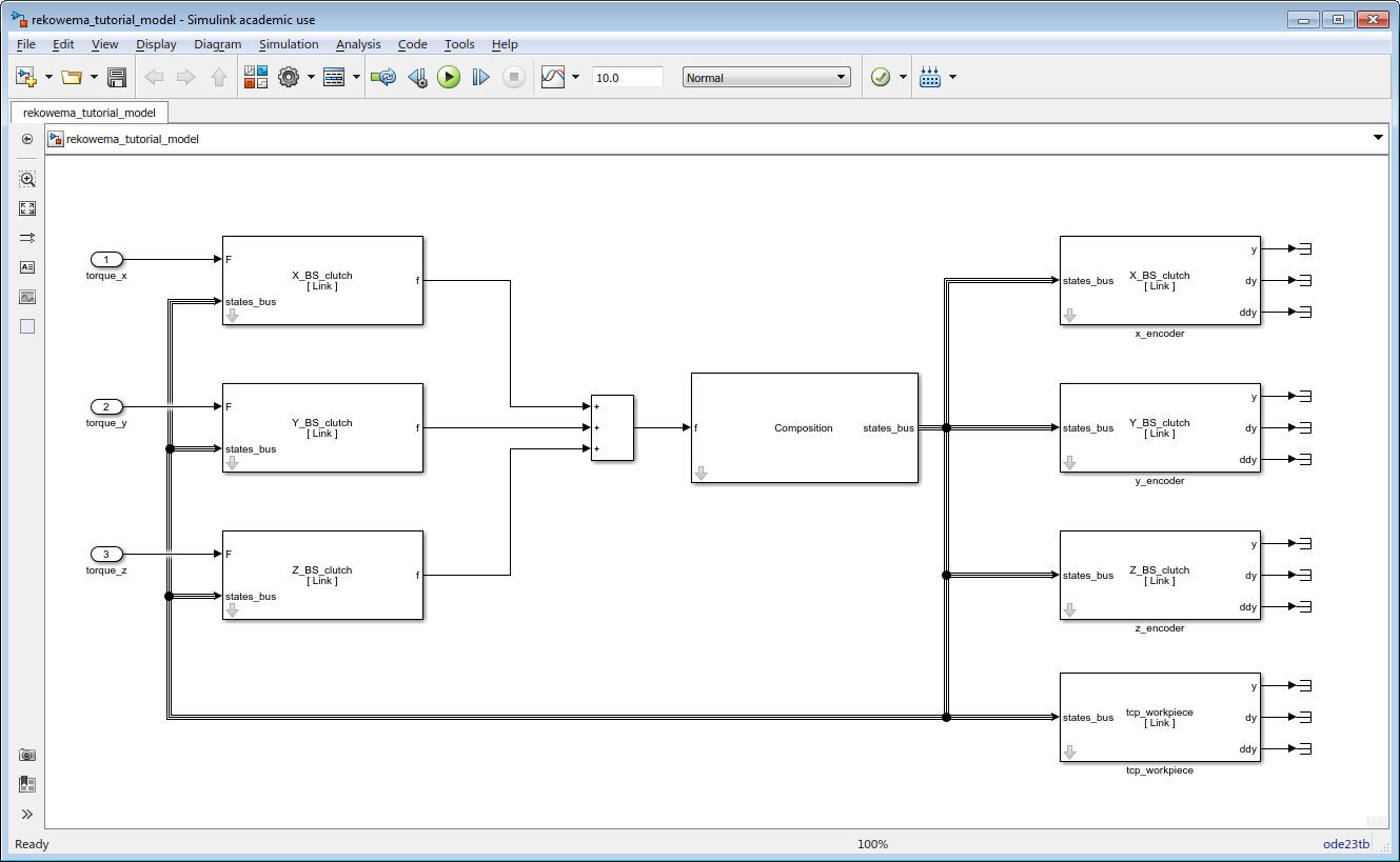
1. Next, add some outputs. Drag a Link output block to your model, rename it to x_encoder, open it, select X_BS_clutch, and tick the ru-direction only. Add some Terminator blocks to the outputs and connect the input to the composition block. Repeat for the other axis. Also add a Link output block for the TCP - workpiece evaluation. Tick all directions for this block. Save the model.

   
   
   

2. In the MATLAB script, input the code for creation of a linearised model from the simulink model and to calculate the frequency response functions.

   %% Create a linearised model
   w = logspace(1,log10(3000),500);
   
   lin_model = Linsys('rekowema_tutorial_model');
   lin_model.add_linio('torque_x', 1, 'input');
   lin_model.add_linio('torque_y', 1, 'input');
   lin_model.add_linio('torque_z', 1, 'input');
   lin_model.add_linio('x_encoder', 2, 'output');
   lin_model.add_linio('y_encoder', 2, 'output');
   lin_model.add_linio('z_encoder', 2, 'output');
   lin_model.add_linio('tcp_workpiece', 2, 'output');
   lin_model.linearise(w)
   % lin_model.save_states([datestr(now, 'yyyymmdd_HHMMSSFFF'), '_freqresults.zip'])
   

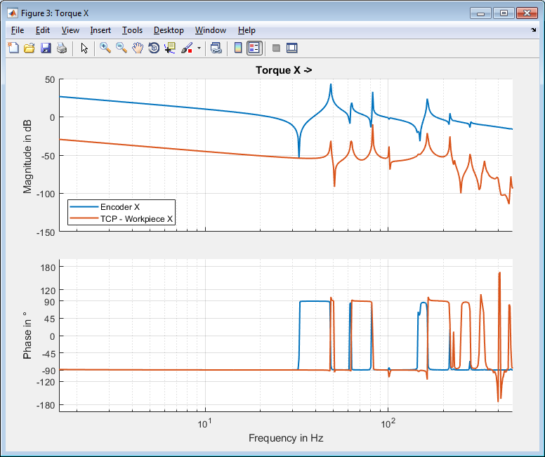
   Add the code for plotting the Bode diagrams.

   %% Create Bode Plots
   % Torque X ->
   figure('name','Torque X');
   lin_model.bode('torque_x', 'x_encoder/2','labels',{'Encoder X'})
   lin_model.bode('torque_x', 'tcp_workpiece/2(1)','labels',{'TCP - Workpiece X'},'colorIndex',2)
   legend show
   title('Torque X -> ')
   
   % Torque Y ->
   figure('name','Torque Y');
   lin_model.bode('torque_y', 'y_encoder/2','labels',{'Encoder Y'})
   lin_model.bode('torque_y', 'tcp_workpiece/2(2)','labels',{'TCP - Workpiece Y'},'colorIndex',2)
   legend show
   title('Torque Y -> ')
   
   % Torque Z ->
   figure('name','Torque Z');
   lin_model.bode('torque_z', 'z_encoder/2','labels',{'Encoder Z'})
   lin_model.bode('torque_z', 'tcp_workpiece/2(3)','labels',{'TCP - Workpiece Z'},'colorIndex',2)
   legend show
   title('Torque Z -> ')
   

   Execute the Create Bode Plots cell to plot the open loop frequency response for the axes.